博文
PCNM动画展示:生态学与空间统计学
||||
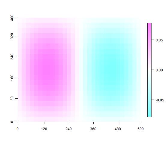
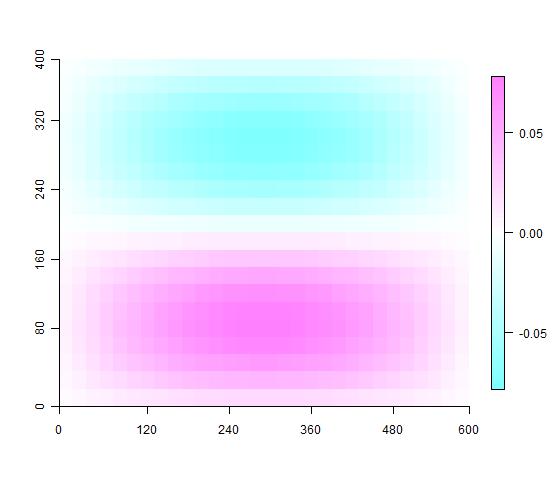
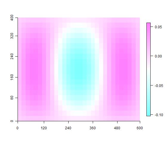
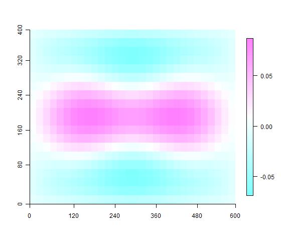
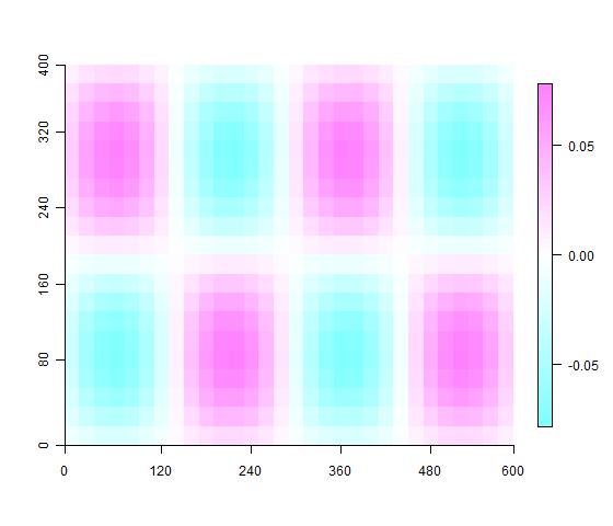
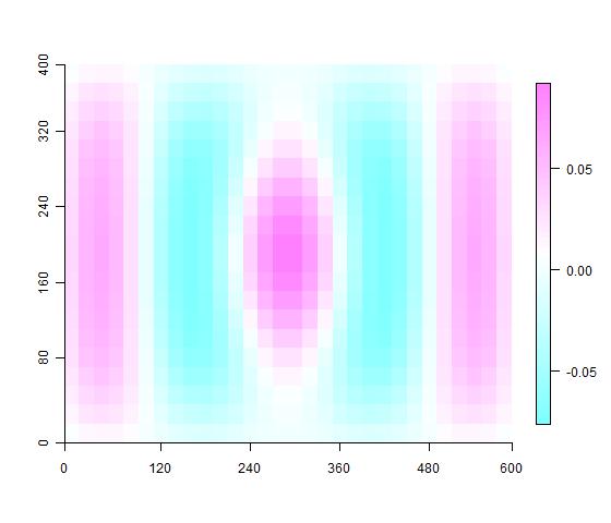
PCNM (Principal Coordinates of Neighbourhood Matrix)是Legendre教授等开发出的表示空间关系的方法,类似于pcoa。常用于生物多样性空间格局研究中,例如在古田山beta多样性研究中,Legendre(2009)就使用了这种方法。用样地的规则栅格距离可以对点两两之间的距离关系进行PCNM模拟。 这里用到了vegan程序包将距离矩阵转换成PCNM的特征向量,用imagevect函数绘制PCNM特征向量在样地中的分布。希望对有兴趣的研究人员有帮助。
将以下代码在R中运行即可。
#### Function imagevect
#### By Jinlong Zhang  <Jinlongzhang01@gmail.com>
#### Institute of Botany, the Chinese Academy of Sciences, Beijing ,China
#### Aug. 18, 2011

imagevect <- function (x, labels, contour = FALSE, gridsize = 20,
                        axes = TRUE, nlabx = 5, nlaby = 5, ...)
{
    require(fields)
   dimension <- function(x, unique = FALSE, sort = FALSE){
        ncharX <- substring(x, 2, regexpr("Y", x)-1)
        ncharY <- substring(x, nchar(ncharX)+3, nchar(x))
        if(unique){
            ncharX = unique(ncharX)
            ncharY = unique(ncharY)
        }
        if(sort){
            ncharX = sort(as.numeric(ncharX))
            ncharY = sort(as.numeric(ncharY))
        }
        res <- list(ncharX, ncharY)
        return(res)
    }

    formatXY <- function(x){
        ncharX <- substring(x, 2, regexpr("Y", x)-1)
        ncharY <- substring(x, nchar(ncharX)+3, nchar(x))
        resX <- c()
        for(i in 1:length(ncharX)){
            n0x <- paste( rep(rep(0, length(ncharX[i])),
                         times = (max(nchar(ncharX)) - nchar(ncharX[i]) + 1)),
                         collapse = "", sep = "")
            resX[i] <- paste("X", substring(n0x, 2, nchar(n0x)), ncharX[i], collapse = "", sep = "")
        }
        resY <- c()
        for(i in 1:length(ncharY)){
            n0x <- paste( rep(rep(0, length(ncharY[i])),
                         times = (max(nchar(ncharY)) - nchar(ncharY[i]) + 1)),
                         collapse = "", sep = "")
            resY[i] <- paste("Y", substring(n0x, 2, nchar(n0x)), ncharY[i], collapse = "", sep = "")
        }
        res <- paste(resX, resY, sep = "")
        return(res)
    }

    sort.x <- x[order(formatXY(labels))]
    rrr <- dimension(labels, unique = TRUE, sort = TRUE)
    dims <- c(length(rrr[[2]]), length(rrr[[1]]))
    dim(sort.x) <- dims
    par(xaxs = "i", yaxs = "i")
    image.plot(nnn <- t(sort.x), axes = FALSE, ...)

    if (contour) {
        contour(nnn, add = TRUE, ...)
    }

    if (axes) {
        points(0, 0, pch = " ", cex = 3)                      ## invoke the large plot

     get.axis.ticks <-
              function(nlabs = NULL, gridsize = NULL, limit_max = NULL){

         ngrid <- (limit_max-0)/gridsize                      ## Obtain number of labels to plot
         per_grid <- 1/(ngrid-1)                              ## Obtain length for each grid
         start <- 0 - (1/(ngrid-1))/2                         ## starting point for the ticks
         stop <- 1 + (1/(ngrid-1))/2                          ## stopping point for the ticks

         lab <-(0:nlabs*(limit_max/nlabs))
         at <- seq(from = start, to = stop,
                   by = ((1 + per_grid))/((length(lab)-1)))   ## Position of the ticks

         return(list(lab, at))

     }
       xaxis.position <- get.axis.ticks(nlabs = nlabx, gridsize = gridsize,
                                limit_max = gridsize * nrow(nnn))
       yaxis.position <- get.axis.ticks(nlabs = nlaby, gridsize = gridsize,
                                limit_max = gridsize * ncol(nnn))

        axis(1, labels = xaxis.position[[1]], at = xaxis.position[[2]])
        axis(2, labels = yaxis.position[[1]], at = yaxis.position[[2]])
    }
    invisible(nnn)
}

library(vegan)

## 模拟一套数据
X <- seq(10, 590, by = 20)
Y <- seq(10, 390, by = 20)

## Label
XY <- expand.grid(X, Y)
names <- paste("X", (XY[,1] + 10)/20 ,"Y", (XY[,2] + 10)/20 , sep = "")
rownames(XY) <- names
## 计算样方两两之间的距离
distXY <- dist(XY)

## 进行pcnm
gtsPCNM <- pcnm(distXY)
head(gtsPCNM$vectors)

## 绘制pcnm图
for(i in 1:10){
    imagevect(gtsPCNM$vectors[,i], labels = names,
               col = topo.colors(100))
    Sys.sleep(0.3)
}


https://m.sciencenet.cn/blog-255662-469451.html
上一篇:Tortoise SVN管理本地代码
下一篇:如何撰写生态学科研论文?