博文
简谐近似、准/非简谐近似:零点能、振动光谱、声子态密度的计算
|||
关注:
1) 零点能的物理意义及影响因素
2) 声子态密度的计算(PDOS)
3) 简谐近似(HA)、准简谐近似(QHA)、非简谐近似
https://atztogo.github.io/phonopy/qha.html
https://en.wikipedia.org/wiki/Quasi-harmonic_approximation
http://physics.nyu.edu/grierlab/elastic7b/node4.html
摘录:
https://www.physicsforums.com/threads/zero-point-energy-dark-energy-and-space.394459/
Long story short, and a lot of simplification, it means that the ground state for the vacuum for electromagnetic fields has a non-zero energy
摘录2:
http://www.baike.com/wiki/%E6%8C%AF%E5%8A%A8%E5%85%89%E8%B0%B1
 谐振子势能曲线和能级图图册
分子振动能级间隔较大,约为0.05-leV. 振动跃迁通常伴有转动跃迁,称为振-转光谱,每一条振动谱带中包含若干条转动谱线. 液态和固态样品中分子间作用较强, 或者由于仪器记录范围较宽、分辨率较低,往往分辨不出振动谱带中的转动谱线,一个谱带就呈现为一个峰. 分子中有多种振动跃迁,整个分子的振动光谱包含若干条谱带.
分子振动可能引起分子固有偶极矩的变化,也可能引起分子极化率的变化. 这两种变化可以分别产生红外光谱和拉曼光谱. 其中, 红外吸收位于近红外和中红外区.
谐振子模型: 对于双原子分子的振动, 也有一种简化处理——谐振子模型.
设双原子分子的两个原子核在平衡距离re (即键长)附近往复振动, 回复力服从虎克定律, 由此可以写出势能V的算符, 与动能T的算符一起构成总能量的哈密顿算符, 进而写出Schrodinger方程:
 方程图册
方程图册
 振动能级图册
振动量子数v=0的能量就是零点能E0,这是一种量子效应, 说明分子即使在无限接近0K时振动也不停息. 这是测不准原理的一种表现.
谐振子能级是振动量子数v的一次函数,故振动能级是等间隔的,间隔为hv.
谐振子振动跃迁选律
振动跃迁也受整体选律和具体选律的限制.
整体选律:只有能够引起分子固有偶极矩变化的振动方式才可能观察到红外光谱. 这对多原子分子也是适用的. 极性分子的固有偶极矩在分子骨架振动过程中总会发生变化, 所以, 极性分子总有红外光谱. 但是, 能不能反过来说, 非极性分子一定没有红外光谱呢? 只有对非极性的双原子分子才能这样说, 因为它们只有一种不改变分子固有偶极矩变化的伸缩振动. 但不能说非极性的多原子分子也一定没有振动光谱. N个原子组成的分子共有3N-6种简正振动方式(直线形分子有3N-5种), 每一种简正振动是否可能具有红外活性, 应由整体选律来考察(这与任何非极性分子都没有转动光谱是不同的).
例如, 苯是12个原子组成的非极性分子, 它有30种简正振动方式, 其中有许多种能够引起分子固有偶极矩变化, 可观察到红外光谱. 但有一些振动方式就没有红外活性,例如,有一种“呼吸振动”就没有红外活性,因为这种振动不会引起分子固有偶极矩变化.
具体选律:才有Δv=±1的跃迁是允许的.
谐振子能级是等间隔的,间隔为hv. 再考虑到具体选律只允许Δv=±1的跃迁, 可以得出结论: 即使分子分布在多种振动能级上, 它们跃迁时也都对应着相同的能量吸收, 因而只有一个振动峰(若考虑其中包含的多条转动谱线, 就是一条谱带). 实际上, 振动能级间隔较大, 室温下大部分分子处于振动基态, 因而主要是v=0到v=1的跃迁.
实验表明这一推断基本是正确的, 确实只有一条很强的基本谱带; 但推断又不完全正确, 因为还发现了一些波数近似等于基本谱带整数倍而强度迅速衰减的泛音谱带. 这一现象表明谐振子模型有缺陷.
不难想象, 分子不可能是完全的谐振子, 而应当是非谐振子. 因为谐振子的抛物形势能曲线暗示着: 分子的核间距无论拉到多长, 化学键也不会被破坏. 至少这一点肯定是不真实的. 所以, 让我们再看看非谐振子模型.
 苯分子的“呼吸振动”图册
") 非谐振子势能曲线和能级图 (D0=De-E0)图册
非谐振子势能曲线和能级图 (D0=De-E0)图册
非谐振子模型:对于非谐振子模型提出过几种势能函数, 例如
 公式图册
公式图册由此建立振动方程,解出的振动能级不再等间隔:
 公式图册
公式图册
式中x为非谐性系数.
非谐振子的整体选律与谐振子相同, 但具体选律却允许Δv=±1,±2,±3,……的跃迁.
考虑到室温下大部分分子处于v=0的振动基态, 可导出从v=0跃迁到任一高能级v的吸收波数公式, 很好地解释了实验上观察到的基本谱带和泛音谱带:
 公式图册
公式图册
其中, 从v=0跃迁到v=1是基本谱带, 而v=0跃迁到v=2、3、4、…分别是第一、第二、第三、…泛音带.
注意:
(1)由于此处低能级的振动量子数已指定为0, 所以, 这里的波数公式都是以高能级的振动量子数v标记的, 这不同于多数情况下用较低能级量子数作为下标的习惯;
(2)由于非谐振子振动波数公式中包含着谐振子振动波数, 这里将非谐振子和谐振子振动波数分别加下标v和e区分.
振动激发可以同时伴随转动激发,用高分辨率红外光谱仪可观察到振转光谱. 例如, HCl的振转光谱如下:
 HCl的振转光谱图册
左侧谱带波数较小, 称为P支; 右侧谱带波数较大, 称为R支. 它们都包含一组间隔为2B的谱线. 中间位置本来有一条称为Q支的谱带, 但对于Σ电子态, Q支是禁阻的, 所以观察不到. 转动谱线为双重线是因为样品中含25%的H37Cl, 产生了向低波数方向的同位素位移.
用振转能级图结合跃迁选律, 很容易解释振转谱带是如何产生的:当振动激发同时伴随转动激发时,若高振动态的转动量子数比低振动态的转动量子数小1, 产生波数较小的P支; 若高振动态的转动量子数比低振动态的转动量子数大1, 产生波数较大的R支.
注意: P支与R支都是针对谱带位置而言, 至于ΔJ = -1或+1, 则由吸收或发射而定. 通常教科书中说P支和R支分别由ΔJ = -1和+1的转动谱线组成, 这只对吸收光谱才成立. 当然, 分子光谱主要使用吸收光谱.
 HCl振转能级图与振转谱带示意图图册
N原子分子有3N个自由度, 其中有3个属于平动, 3个属于转动(直线形分子为2个), 剩余的3N-6个为振动自由度. 每个振动自由度有一种称之为正则振动或简正振动的运动方式: 所有原子以同频率、同位相振动,同时通过平衡点、同时到达极大值. 正则振动方式可以用群论的方法处理, 由投影算符给出. 每种正则振动方式有一个特征频率, 并可从理论上计算出来.
多原子分子的振动非常复杂. 原则上, 任何复杂振动都可以分解为正则振动的叠加, 实际上, 多原子分子的振动光谱很少直接使用纯粹的理论计算来解析, 而多用经验规律解析. 但近年来, 计算化学中光谱模拟软件发展很快, 对于光谱的辅助解析作用值得重视.
一般说来, 化学键的伸缩振动频率大于弯曲振动频率, 重键振动频率大于单键振动频率, 连接较轻的原子(如H)的化学键振动频率较高.
频率较高的振动不易受其它因素影响, 能保留自己的特征. 经验表明, 官能团具有相对稳定的特征频率, 因此, 尽管任何振动方式原则上都是所有原子参与, 但同一种官能团的振动频率在不同化合物中大致相同, 据此可以鉴别不同类型的化合物.
频率较低的振动则很容易随环境而变, 特征性很差, 分子结构的细微差别就能引起这种振动的变化, 因此反映的是每一种具体分子的结构信息, 犹如人的指纹,这种振动出现的区域也就称为“指纹区”.
IR谱的扫描范围通常在4000-650cm-1, 特征频率与指纹区大致以1500cm-1为界:
(1)特征频率区4000 ~ 1500cm-1, 又可分成两个小区: 波数较高一端是与氢原子相结合的官能团,如OH、NH、CH键伸缩振动吸收带(C-H、 N-H、 O-H, ~3000 cm-1); 波数较低一端是叁键、双键和累积双键如C=C=C的吸收带(叁键 ~2100 cm-1;双键,1600-1700 cm-1).
(2)指纹区1500-650cm-1:这是单键伸缩振动和弯曲振动吸收(单键C-C、C-N、C-O,800-900 cm-1) .
解析红外光谱时可以查阅光谱手册, 其中有详尽的特征频率表;若样品已被研究过,则可通过索引查阅各种图谱集,或查网上数据库来对照. 一般说来,红外光谱完全相同的物质是同一种物质,只有对映异构体和少数大分子同系物是例外.
解析红外光谱的基本步骤
红外光谱对鉴别官能团、测定分子结构具有重要作用,但解释复杂分子的红外光谱并不容易,除了懂得基本原理外,更需要比较丰富的实践经验. 初学者可以选择一些比较简单的分子作为练习,但不要急于很快取得成功.
(1) 根据化合物的分子式写出各种可能的结构式.
(2) 按照特征频率表,对整个光谱图认真检查, 看看有哪些官能团和骨架的特征峰,如N-H、O-H、C=O、烯基、芳环等.
(3) 检查C-H伸缩区域 (2700-3300cm-1),辨别是否有不饱和或芳香环:
饱和烃的C-H伸缩一般不超过3000cm-1;
烯烃的C-H伸缩有对称与反对称之分: 前者在2975cm-1处, 往往与饱和烃甲基反对称伸缩重叠; 后者在3080cm-1处, 是烯烃的特征,但应注意芳烃C-H、卤代烷、小环环烷的C-H伸缩也在此区;
芳烃的C-H伸缩在3030cm-1附近;
再检查1360-1380cm-1区域,看是否有-CH2-和-CH3.
(4) 若化合物除C、H、O外,还有其它原子X,则寻找X-H或X-C特征峰. 例如,亚胺的N=C伸缩振动峰在1690-1640 cm-1区间,可判别亚胺基是否存在;而含有叁键的氰基C≡N伸缩振动峰在2245cm-1附近,若发生共轭则降低约30 cm-1.
(5) 若化合物不是芳香化合物,则725cm-1附近的宽带表示四个以上的-CH2-基组成的长链.
(6) 继续查找其它特点. 例如,单核芳烃的C=C伸缩振动在1500和1600cm-1附近有两个峰, 一般前者较强后者较弱, 可作为芳核存在的标志,等等.
红外光谱仪
红外光谱仪的光源可用碳化硅棒通过电热发光. 样品池和棱镜等用透红外线的材料(如 NaCI、KBr、LiF等)制作,也可用光栅分光. 热电偶或热敏电阻探测器将讯号传送给放大记录系统.
付里叶变换红外光谱简介
傅里叶变换红外光谱仪是非色散型光谱仪,其核心部分是一台双光束干涉仪(常用迈克耳孙干涉仪). 当动镜移动时,经过干涉仪的两束相干光的光程差改变,到达探测器的光强随之改变,得到干涉图,再经傅里叶变换得到光谱.
傅里叶变换光谱仪的主要优点是:多道测量提高了信噪比;没有入射、出射狭缝限制,光通量高使仪器灵敏度提高;以氦、氖激光波长为标准,波数值精确度可达0.01cm-1 ; 增加动镜移动距离可提高分辨率;工作波段从可见区可延伸到毫米区,实现远红外光谱测定.
分子振动也可能引起分子极化率的变化,产生拉曼光谱. 拉曼光谱不是观察光的吸收, 而是观察光的非弹性散射, 因此光源的频率不必与振动跃迁对应的频率相一致, 例如用可见或紫外光源照射在样品上,在垂直于入射光的方向,观测散射光的强度随波长的变化关系,非弹性散射峰频率和弹性散射峰频率(即入射光频率)之差反映出分子的振动转动能级. 非弹性散射光很弱,故拉曼光谱过去较难观测. 激光拉曼光谱的出现使灵敏度和分辨力大大提高,应用日益广泛.
拉曼现象可以在各种入射光频率下发生(例如用波长为632.8 nm 的He-Ne 激光).拉曼光谱由于产生机理和红外光谱不同,在选律方面也不相同.
光子与分子碰撞时, 少部分在侧向散射. 其中, 又有大部分是频率不变的弹性散射, 少部分是频率增大或减小的非弹性散射. 频率增减是由于非弹性散射时光子与分子交换能量引起的,频率减小和增大分别产生Stokes线与反Stokes线.
对于有对称中心的分子, 任何一种振动方式都不会在红外与拉曼光谱上都观察到, 称为互斥规则. 研究分子结构时二者可以互补. 根据群论知识容易明白:光谱强度与下列矩阵元平方成正比. 为保证矩阵元不为零,被积函数的宇称必须为g. 红外光谱的跃迁矩算符为u宇称的偶极矩算符, 而拉曼光谱的跃迁矩算符为G宇称的极化率算符. 由于大多数分子的始态ψi为g宇称,所以,跃迁的终态ψj在红外与拉曼光谱上的宇称必须分别是u和g:
 公式图册
公式图册零点振动能
摘录3:
http://en.wikipedia.org/wiki/Zero-point_energy
Zero-point energy
Zero-point energy, also called quantum vacuum zero-point energy, is the lowest possible energy that a quantum mechanicalphysical system may have; it is the energy of its ground state. All quantum mechanical systems undergo fluctuations even in their ground state and have an associated zero-point energy, a consequence of their wave-like nature. The uncertainty principle requires every physical system to have a zero-point energy greater than the minimum of its classical potential well. This results in motion even at absolute zero. For example, liquid helium does not freeze under atmospheric pressure at any temperature because of its zero-point energy.
The concept of zero-point energy was developed in Germany by Albert Einstein and Otto Stern in 1913, as a corrective term added to a zero-grounded formula developed by Max Planck in 1900.[1][2] The term zero-point energyoriginates from the German Nullpunktsenergie.[1][2] An alternative form of the German term is Nullpunktenergie (without the s).
Vacuum energy is the zero-point energy of all the fields in space, which in the Standard Model includes the electromagnetic field, other gauge fields, fermionic fields, and the Higgs field. It is the energy of the vacuum, which in quantum field theory is defined not as empty space but as the ground state of the fields. In cosmology, the vacuum energy is one possible explanation for the cosmological constant.[3] A related term is zero-point field, which is the lowest energy state of a particular field.[4]
In 1900, Max Planck derived the formula for the energy of a single energy radiator, e.g., a vibrating atomic unit:[5]

where  is Planck's constant,
  is the frequency, k is Boltzmann's constant, and T is the absolute temperature.
Then in 1913, using this formula as a basis, Albert Einstein and Otto Stern published a paper in which they suggested for the first time the existence of a residual energy that all oscillators have at absolute zero. They called this residual energy Nullpunktsenergie (German), later translated as zero-point energy. They carried out an analysis of the specific heat of hydrogen gas at low temperature, and concluded that the data are best represented if the vibrational energy is[1][2]
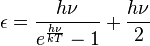
According to this expression, an atomic system at absolute zero retains an energy of ½hν.
Relation to the uncertainty principle[edit]Zero-point energy is fundamentally related to the Heisenberg uncertainty principle.[6] Roughly speaking, the uncertainty principle states that complementary variables (such as a particle's position and momentum, or a field's value and derivative at a point in space) cannot simultaneously be defined precisely by any given quantum state. In particular, there cannot be a state in which the system sits motionless at the bottom of its potential well, for then its position and momentum would both be completely determined to arbitrarily great precision. Therefore, the lowest-energy state (the ground state) of the system must have a distribution in position and momentum that satisfies the uncertainty principle, which implies its energy must be greater than the minimum of the potential well.
Near the bottom of a potential well, the Hamiltonian of a system (the quantum-mechanical operator giving its energy) can be approximated as

where  is the minimum of the classical potential well. The uncertainty principle tells us that
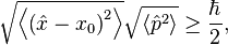
making the expectation values of the kinetic and potential terms above satisfy
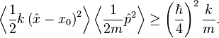
The expectation value of the energy must therefore be at least
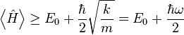
where  is the angular frequency at which the system oscillates.
A more thorough treatment, showing that the energy of the ground state actually is  requires solving for the ground state of the system. See quantum harmonic oscillator for details.
The concept of zero-point energy occurs in a number of situations.
In ordinary quantum mechanics, the zero-point energy is the energy associated with the ground state of the system. The professional physics literature tends to measure frequency, as denoted by above, using angular frequency, denoted with  and defined by =
  . This leads to a convention of writing Planck's constant with a bar through its top (
 ) to denote the quantity /
 . In those terms, the most famous such example of zero-point energy is
  associated with the ground state of the quantum harmonic oscillator. In quantum mechanical terms, the zero-point energy is the expectation value of the Hamiltonian of the system in the ground state.
In quantum field theory, the fabric of space is visualized as consisting of fields, with the field at every point in space and time being a quantum harmonic oscillator, with neighboring oscillators interacting. In this case, one has a contribution of from every point in space, resulting in a calculation of infinite zero-point energy in any finite volume; this is one reason renormalization is needed to make sense of quantum field theories. The zero-point energy is again the expectation value of the Hamiltonian; here, however, the phrase vacuum expectation value is more commonly used, and the energy is called the vacuum energy.
In quantum perturbation theory, it is sometimes said that the contribution of one-loop and multi-loop Feynman diagrams to elementary particlepropagators are the contribution of vacuum fluctuations or the zero-point energy to the particle masses.
Experimental observations[edit]A phenomenon that is commonly presented as evidence for the existence of zero-point energy in vacuum is the Casimir effect, proposed in 1948 by DutchphysicistHendrik B. G. Casimir (Philips Research), who considered the quantized electromagnetic field between a pair of grounded, neutral metal plates. The vacuum energy contains contributions from all wavelengths, except those excluded by the spacing between plates. As the plates draw together, more wavelengths are excluded and the vacuum energy decreases. The decrease in energy means there must be a force doing work on the plates as they move. This force has been measured and found to be in good agreement with the theory. However, there is still some debate on whether vacuum energy is necessary to explain the Casimir effect. Robert Jaffe of MIT argues that the Casimir force should not be considered evidence for vacuum energy, since it can be derived in QED without reference to vacuum energy by considering charge-current interactions (the radiation-reaction picture).[7]
The experimentally measured Lamb shift has been argued to be, in part, a zero-point energy effect.[8]
Gravitation and cosmology[edit]| Why doesn't the zero-point energy density of the vacuum change with changes in the volume of the universe? And related to that, why doesn't the large constant zero-point energy density of the vacuum cause a large cosmological constant? What cancels it out? |
In cosmology, the zero-point energy offers an intriguing possibility for explaining the speculative positive values of the proposed cosmological constant. [9] In brief, if the energy is "really there", then it should exert a gravitational force.[10] In general relativity, mass and energy are equivalent; both produce a gravitational field. One obvious difficulty with this association is that the zero-point energy of the vacuum is absurdly large. Naively, it is infinite, because it includes the energy of waves with arbitrarily short wavelengths. But since only differences in energy are physically measurable, the infinity can be removed by renormalization. In all practical calculations, this is how the infinity is handled. It is also arguable[original research?] that undiscovered physics relevant at the Planck scale reduces or eliminates the energy of waves shorter than the Planck length, making the total zero-point energy finite.[citation needed]
Utilization controversy[edit]As a scientific concept, the existence of zero-point energy is not controversial. However, the ability to harness zero point energy for useful work is considered pseudoscience by the scientific community at large.[11][12]
Over the years, there have been numerous claims of devices capable of extracting usable zero-point energy. None of the claims have ever been confirmed by the scientific community, and most of these claims are dismissed by physicists and engineers after third-party inspection of such a device or based on disbelief in the viability of a technical design and theoretical corroboration.[13]
Science skeptic and writer, Martin Gardner has called claims of such zero-point-energy-based systems, "as hopeless as past efforts to build perpetual motion machines"[14]Perpetual motion machine refers to technical designs of machines that can operate indefinitely, optionally with additional output of excessive energy, without any cited input source of energy, which is in violation of the laws of thermodynamics. Formally, technical designs that claim to harness zero-point energy would not fall into this category, while zero-point energy is claimed as the input source of energy. However, in popular science it is common[weasel words] to disregard whether such a technical claim deviates first and foremost from the laws of thermodynamics, or from the theories of quantum mechanics. Despite the scientific stance to typically discount the claims, numerous articles and books have been published addressing and discussing the potential of tapping zero-point-energy from the quantum vacuum or elsewhere. Examples of such are the work of the following authors: Claus Wilhelm Turtur,[15] Jeane Manning, Joel Garbon,[16] John Bedini,[17] Tom Bearden,[18][19][20] Thomas Valone,[21][22][23] Moray B King,[24][25][26] Christopher Toussaint, Bill Jenkins,[27]Nick Cook[28] and William James.[29]
In quantum theory, zero-point energy is a minimum energy below which a thermodynamic system can never go.[11] Thus, none of this energy can be withdrawn without altering the system to a different form in which the system has a lower zero-point energy. One of the hypotheses that claims that zero-point energy is infinite is stochastic electrodynamics. In it, the zero-point field is viewed as simply a classical background isotropic noise wave field which excites all systems present in the vacuum and thus is responsible for their minimum-energy or "ground" states. The requirement of Lorentz invariance at a statistical level then implies that the energy density spectrum must increase with the third power of frequency, implying infinite energy density when integrated over all frequencies.[30]
According to a NASA contractor report, "the concept of accessing a significant amount of useful energy from the ZPE gained much credibility when a major article on this topic was published in Aviation Week & Space Technology (March 1st, 2004), a leading aerospace industry magazine".[31]
The calculation that underlies the Casimir experiment, a calculation based on the formula predicting infinite vacuum energy, shows the zero-point energy of a system consisting of a vacuum between two plates will decrease at a finite rate as the two plates are drawn together. The vacuum energies are predicted to be infinite, but the changes are predicted to be finite. Casimir combined the projected rate of change in zero-point energy with the principle of conservation of energy to predict a force on the plates. The predicted force, which is very small and was experimentally measured to be within 5% of its predicted value, is finite.[32] Even though the zero-point energy is theoretically infinite, there is as yet no evidence to suggest that infinite amounts of zero-point energy are available for use, that zero-point energy can be withdrawn for free, or that zero-point energy can be used in violation of conservation of energy.[33]
In the contrary of energy generation, a field of study where there is a somewhat realistic potential for the utilization of zero-point energy might be in the design of extremely small scale devices like MEMS and NEMS or in distant futuristic propulsion technology of extremely long-distance space-travel.[11]
A document released by the NGIC shows there is ongoing worldwide research into zero-point energy, particular in China, Germany, Russia and Brazil. An analyst of the Defense Intelligence Agency has indicated that research into successfully harnessing zero-point energy for energy generation purposes is a serious concern inside the intelligence community.[11]
In popular culture[edit]In 1986, Arthur C. Clarke published a science fiction novel called The Songs of Distant Earth which depicts a starship called Magellan that is powered by the quantum vacuum zero point energy.
In Disney/Pixar's animated film The Incredibles, the main villain Syndrome refers to his weapons as using zero-point energy.[34][35] The fan fiction community devoted to the character is named "Zero Point" because of this.[36]
In the critically acclaimed game from Valve Corporation, Half-Life 2, a "zero-point energy field manipulator" (popularly known as a "gravity gun"), meant to handle sensitive, anomalous and hazardous materials, is used as both a weapon to throw objects at enemies in high speeds, as a primary attack, and a tool to solve physics puzzles consisting in moving objects of considerable weight.
In Nintendo's Star Fox series, there are mentions of a "G-Diffusion" system. The so-called G-diffusion is an experimental power system used in the game's starfighters that reduces gravity forces on the pilot and provides a respectable power source for shields and propulsion, using advanced zero-point energy technology.
In the webcomic Schlock Mercenary, a major running plot-point centers around an enormous zero-point energy generator built from the super massive black hole comprising the core Milky Way Galaxy.
In the popular science-fiction programs generally labeled under Stargate SG-1, the intergalactic colonists visiting Atlantis often refer to and make use of "ZPMs" shortened from "Zero-Point Modules." Although fantastically powerful in terms of available energy density, these fictional energy sources still dissipate over time which the example of Helium's non-solid state proves inaccurate.
| 如果你用的是简谐近似(Harmonic approximation)的话ISIF=3,如果你用的是准简谐近似(Quasi-harmonic approximation)ISIF=4.好好看看PHONO的说明书吧。还有就是有关软件的说明书。不知道你用的是哪款计算声子的软件?还是MS里面的? |
理论上,QHA比HA多考虑了一个体积效应。
https://atztogo.github.io/phonopy/qha.html
Using phonopy results of thermal properties, thermal expansion and heat capacity at constant pressure can be calculated under the quasi-harmonic approximation. phonopy-qhais the script to calculate them. An example of the usage for example/Si-QHA is as follows.
To watch selected plots:

Without plots:
1st argument is the filename of volume-energy data (in the above expample, e-v.dat). The volume and energy of the unit cell (default units are in and eV, respectively). An example of the volume-energy file is:
Here the word ‘quasi-harmonic approximation’ is used for an approximation that introduces volume dependence of phonon frequencies as a part of anharmonic effect.
A part of temperature effect can be included into total energy of electronic structure through phonon (Helmholtz) free energy at constant volume. But what we want to know is thermal properties at constant pressure. We need some transformation from function of V to function of p. Gibbs free energy is defined at a constant pressure by the transformation:
where
means to find unique minimum value in the brackets by changing volume. Since volume dependencies of energies in electronic and phonon structures are different, volume giving the minimum value of the energy function in the square brackets shifts from the value calculated only from electronic structure even at 0 K. By increasing temperature, the volume dependence of phonon free energy changes, then the equilibrium volume at temperatures changes. This is considered as thermal expansion under this approximation.
phonopy-qha collects the values at volumes and transforms into the thermal properties at constant pressure.
https://en.wikipedia.org/wiki/Quasi-harmonic_approximation
The quasi-harmonic approximation expands upon the harmonic phonon model of lattice dynamics. The harmonic phonon model states that all interatomic forces are purely harmonic, but such a model is inadequate to explain thermal expansion, as the equilibrium distance between atoms in such a model is independent of temperature.
Thus in the quasi-harmonic model, from a phonon point of view, phonon frequencies become volume-dependent in the quasi-harmonic approximation, such that for each volume, the harmonic approximation holds.
Thermodynamics[edit]For a lattice, the Helmholtz free energy F in the quasi-harmonic approximation is

where U is the internal lattice energy, EZP is the vibrational zero-point energy of the lattice, T is the absolute temperature, V is the volume and S is the entropy due to the vibrational degrees of freedom. The specific definition of the volume is of no particular importance, as long as the definition is used consistently throughout. It can be the volume per primitive unit cell, volume per conventional unit cell, or even molar volume. This choice does not affect the following in any way.
The zero-point energy term equals

where N is the number of terms in the sum, k is a wave vector, i denotes a phonon band, h is Planck's constant and νk,i(V) is the frequency of a phonon with wave vector k in thei-th band at volume V.
The entropy term equals
![{.displaystyle S(V)=-{.frac {1}{N}}.sum _{.mathbf {k} ,i}k_{B}.ln .left[1-.exp .left(-{.frac {h.nu _{.mathbf {k} ,i}(V)}{k_{B}T}}.right).right]+{.frac {1}{N}}.sum _{.mathbf {k} ,i}k_{B}{.frac {h.nu _{.mathbf {k} ,i}(V)}{k_{B}T}}.left[.exp .left({.frac {h.nu _{.mathbf {k} ,i}(V)}{k_{B}T}}.right)-1.right]^{-1}}](https://wikimedia.org/api/rest_v1/media/math/render/svg/c88575f6108c96aa8947b7058d697e4ded6d7796)
where kB is the Boltzmann constant. The frequency ν as a function of k is the dispersion relation. Note that for a constant value of V, these equations corresponds to that of the harmonic approximation.
By applying a Legendre transform, it is possible to obtain the Gibbs free energy G of the system as a function of temperature and pressure.
![G(T,P)=.min _{V}.left[U(V)+E_{{ZP}}(V)-TS(T,V)+PV.right]](https://wikimedia.org/api/rest_v1/media/math/render/svg/aae8a07f1c24d994a3de0962f79582eb5efa70b0)
Where P is the pressure. The minimal value for G is found at the equilibrium volume for a given T and P.
https://m.sciencenet.cn/blog-567091-842189.html
上一篇:学术兴趣小组之QQ群的使用
下一篇:简单物质不简单-从H2O说起