博文
微生物菌群CDA与RDA分析
||
参考来自宏基因组https://mp.weixin.qq.com/s?src=11×tamp=1612576794&ver=2873&signature=jWvM0w2wPnqc44STYsN09yIp5mGZL6Uu16vy0c0LIQ6JH5f8Sz-QXEd*BZgV0qi3zNI17KrSkwYeUuTj*Zv7VKuaqzJ0KFpI9kqTMI4kuCRLVBX-WjuChnhBUBHl*MYJ&new=1
# 首先要安装devtools包,仅需安装一次
install.packages("devtools")
# 加载devtools包
library(devtools)
# 下载ggvegan包
devtools::install_github("gavinsimpson/ggvegan")
library(ggvegan)
otu.tab <- read.csv("otutab.txt", row.names = 1, header=T, sep="\t")
env.data <- read.csv("new_meta.txt", row.names = 1, fill = T, header=T, sep="\t")
#transform data
otu <- t(otu.tab)
#data normolization (Legendre and Gallagher,2001)
##by log 环境因子进行log转化,以减少同一种环境因子之间本身数值大小造成的影响。
env.data.log <- log1p(env.data)##
##delete NA 删掉空值行
env <- na.omit(env.data.log)
###hellinger transform OTU进行hellinger转化,使数据均一性更好。
otu.hell <- decostand(otu, "hellinger")
#DCA analysis   DCA分析看分析结果中Lengths of gradient的第一轴中的Axis lengths大小,
如果大于4.0,就应该选CCA,如果在3.0-4.0之间,选RDA和CCA均可,如果小于3.0,RDA的结果要好于CCA。
本例中,我们数据的Axis lengths 大小为0.63859,所有我们应该选择RDA进行分析
sel <- decorana(otu.hell)
sel
otu.tab.0 <- rda(otu.hell ~ 1, env) #no variables
#Axis 第一项大于四应该用CCA分析
otu.tab.1<- rda(otu.hell ~ ., env)
#我们在筛选完RDA和CCA分析后,我们需要对所有环境因子进行共线性分析,利用方差膨胀因子分析
vif.cca(otu.tab.1)
#删除掉共线性的环境因子,删掉最大的变量,直到所有的变量都小于10
otu.tab.1 <- rda(otu.hell ~ N+P+K+Ca+Mg+pH+Al+Fe+Mn+Zn+Mo, env.data.log)
otu.tab.1
vif.cca(otu.tab.1)
#进一步筛选
otu.tab.1 <- rda(otu.hell ~ N+P+K+Mg+pH+Al+Fe+Mn+Zn+Mo, env.data.log)
vif.cca(otu.tab.1)
#test again
otu.tab.1 <- rda(otu.hell ~ N+P+K+Mg+pH+Fe+Mn+Zn+Mo, env.data.log)
#方差膨胀因子分析,目前所有变量都已经小于10
vif.cca(otu.tab.1)
##用step模型检测最低AIC值
#mod.u <- step(otu.tab.0, scope = formula(otu.tab.1), test = "perm")
# "perm"增加P值等参数
mod.d <- step(otu.tab.0, scope = (list(lower = formula(otu.tab.0),
upper = formula(otu.tab.1))))
mod.d
##本处筛选的结果,找到一个Mg环境因子适合模型构建,为了下一步画图,我们
#保留上述筛选的结果所有非共线性的环境因子
#choose variables for best model and rda analysis again#
(otu.rda.f <- rda(otu.hell ~ N+P+K+Mg+pH+Fe+Mn+Zn+Mo, env))
anova(otu.rda.f)
anova(otu.rda.f, by = "term")
anova(otu.rda.f, by = "axis")
#计算db-rda
otu.tab.bray <- vegdist(otu.hell, "bray")
#dbrda() for dbRDA # cca() for CCA
otu.tab.b<- capscale(otu.tab.bray ~ ., env)
##绘制db-RDA图
plot(otu.tab.b ,display=c("si","bp","sp"))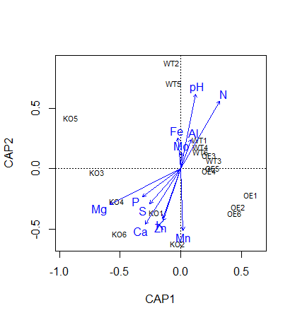
## 用ggvegan绘制RDA图
p1<- autoplot(otu.rda.f, arrows = TRUE,axes = c(1, 2), geom = "text",
layers = c("sites"),
legend.position = "right", title = "db-RDA")
p1
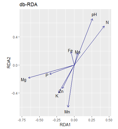
p2<- autoplot(otu.rda.f, arrows = TRUE,axes = c(1, 2), geom = "text",
layers = c("biplot"),
legend.position = "right", title = "db-RDA")
p2
p3<- autoplot(otu.rda.f, arrows = TRUE,axes = c(1, 2), geom = "text",
layers = c("sites","biplot"),
legend.position = "right", title = "db-RDA")
p3
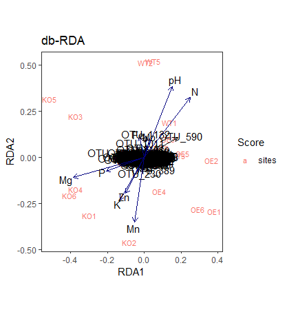
p4<- autoplot(otu.rda.f, arrows = TRUE,axes = c(1, 2),
geom = "text", layers = c( "species","sites",
"biplot", "centroids"), legend.position = "right",
title = "db-RDA")
p4
## 添加图层
p5<-p4 + theme_bw()+theme(panel.grid.major =element_blank(),
panel.grid.minor = element_blank())
p5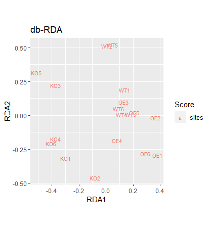


https://m.sciencenet.cn/blog-3448646-1270915.html
上一篇:otu分隔不同归属
下一篇:鸢尾花PCA分析与绘图
扫一扫,分享此博文