A new processing method for the pollen samples from Palaeogene red beds in the Liguanqiao Basin, Hubei Province and Pleistocene loess from the Chinese Loess Plateau Hongyan Xu (徐红艳), Hanchao Jiang* (蒋汉朝*), Xueshun Mai (麦学舜), Xiaolin Ma (马小林) Over the past decade, palynoflora investigation of Tertiary red beds and Pleistocene loess has been the focus of an increasing number of studies. Pollen extraction from sediments is a prerequisite for palynoflora investigation. In this study, we explored a new pollen processing method and successfully extracted a large number of pollen grains from the Palaeogene red beds in the Liguanqiao Basin, Hubei Province and the Pleistocene loess from the southern Chinese Loess Plateau. We present several key steps in our new method. (1) Samples from arid to semi-arid regions are usually well cemented and should be gently crushed and sieved with 30-mesh screen for pollen analysis to maximize the number of pollen grains recovered from sediments. (2) In order to remove organic matter most effectively, samples should be heated until just boiling in ~3% NaOH solution for not more than 5 minutes. (3) The residue after acid-alkali treatment should be dried at 85℃ for 7~9 h to ensure that density of the heavy liquid is not diluted during the next step. (4) The KI heavy liquid, with a density of 1.74-1.76, should be used to concentrate the pollen. (5) Sieving with a 7-μm stainless steel mesh resulted in the loss of few pollen grains. In contrast, sieving with a 10-μm-nylon mesh resulted in loss of many small pollen grains. Importantly, our study extended the first appearance of Artemisia in China back to the Late Palaeocene, and is significant for vegetation reconstruction in the arid to semi-arid regions during the Cenozoic Era. QI2013-Xu and Jiang et al.pdf
A couple of months ago I was working with a bunch of pictures I had taken at home. I had about 40 of them, and I needed to crop and resize them all the same way. Naturally, I wrote a MATLAB script to do it. This experience reminded me that customers sometimes ask "How do I use the Image Processing Toolbox to do batch processing of my images?" Really, though, this isn't a toolbox question; it's a MATLAB question. In other words, the basic MATLAB techniques for batch processing apply to any domain, not just image processing. Contents Step 1: Get a list of filenames Step 2: Determine the processing steps to follow for each file Step 3: Put everything together in a for loop Step 1: Get a list of filenames If you use the dir function with an output argument, you get back a structure array containing the filenames, as well as other information about each file. Let's say I want to process all files ending in .jpg: files = dir( '*.jpg' )files = 42x1 struct array with fields: name date bytes isdir The files struct array has 42 elements, indicating that there are 42 files matching "*.jpg" in the current directory. Let's look at the details for a couple of these files. files(1)ans = name: 'IMG_0175.jpg' date: '12-Feb-2006 10:49:30' bytes: 962477 isdir: 0 files(end)ans = name: 'IMG_0216.jpg' date: '12-Feb-2006 11:09:10' bytes: 1004842 isdir: 0 Step 2: Determine the processing steps to follow for each file There are four basic steps to follow for each file: 1. Read in the data from the file. 2. Process the data. 3. Construct the output filename. 4. Write out the processed data. Here's what my read and processing steps looked like: rgb = imread( 'IMG_0175.jpg' ); % or rgb = imread(files(1).name); rgb = rgb(1:1800, 520:2000, :); rgb = imresize(rgb, 0.2, 'bicubic' ); You have many options to consider for constructing the output filename. In my case, I wanted to use the same name but in a subfolder: output_name = % Use fullfile instead if you want % multiplatform portability output_name = cropped\IMG_0175.jpg Here's another example of output name construction. You might use something like this if you want to change image formats. input_name = files(1).nameinput_name = IMG_0175.jpg = fileparts(input_name)path = '' name = IMG_0175 extension = .jpg output_name = fullfile(path, )output_name = IMG_0175.tif Step 3: Put everything together in a for loop Here's my complete batch processing loop: files = dir( '*.JPG' ); for k = 1:numel(files) rgb = imread(files(k).name); rgb = rgb(1:1800, 520:2000, :); rgb = imresize(rgb, 0.2, 'bicubic' ); imwrite(rgb, ); end amp;lt;emamp;gt;Anbsp;JavaScript-enablednbsp;browsernbsp;isnbsp;requirednbsp;tonbsp;usenbsp;thenbsp;quot;Getnbsp;thenbsp;MATLABnbsp;codequot;nbsp;link.amp;lt;/emamp;gt;nbsp; Get the MATLAB code
Statistical metaphor processing 共54页。 摘要: Metaphor is highly frequent in language, which makes its computational processing indispensable for real-world NLP applications addressing semantic tasks. Previous approaches to metaphor modeling rely on task-specific hand-coded knowledge and operate on a limited domain or a subset of phenomena. We present the first integrated open-domain statistical model of metaphor processing in unrestricted text. Our method first identifies metaphorical expressions in running text and then paraphrases them with their literal paraphrases. Such a text-to-text model of metaphor interpretation is compatible with other NLP applications that can benefit from metaphor resolution. Our approach is minimally supervised, relies on the state-of-the-art parsing and lexical acquisition technologies (distributional clustering and selectional preference induction), and operates with a high accuracy. 下载地址: http://www.pipipan.com/file/22095585
http://plantsinmotion.bio.indiana.edu/plantmotion/movements/leafmovements/clocks.html Interesting movies Plant in motion. Image processing is more and more important for Biology research. I think many people like automatic stuffs.
微波化学值得研究: Microwave chemistry is not “voodoo science”, but in essence an incredibly effective, safe, rapid, and highly reproducible way to perform an autoclave experiment under strictly controlled processing conditions. 但是: Most of today's commercially available laboratory microwave reactors are not very well suited to study microwave effects.These instruments were essentially designed to “rapidly generate compounds”, not to perform accurate kinetic investigations. Therefore, in most instances, these microwave reactors are not equipped with the temperature-sensing technology and software algorithms that are needed to accurately control and monitor reaction temperature during a microwave chemistry experiment (taking all eventualities such as viscosity increases, exothermic behavior, and changes in the microwave absorptivity of the reaction mixture into account). C. Oliver Kappe et al. Microwave Effects in Organic Synthesis—Myth or Reality? Angew. Chem. Int. Ed. 2012 , DOI : 10.1002/anie.201204103 201204103_ftp.pdf
欢迎大家访问OpenPR主页: http://www.openpr.org.cn , 并提出意见和建议!同时,OpenPR也期待您分享您的代码! OpenPR, stands for Open Pattern Recognition project and is intended to be an open source platform for sharing algorithms of image processing, computer vision, natural language processing, pattern recognition, machine learning and the related fields. Code released by OpenPR is under BSD license, and can be freely used for education and academic research. OpenPR is currently supported by the National Laboratory of Pattern Recognition, Institution of Automation, Chinese Academy of Sciences. Thresholding program This is demo program on global thresholding for image of bright small objects, such as aircrafts in airports. the program include four method, otsu,2D-Tsallis,PSSIM, Smoothnees Method. Authorschen xueyun E-mail xueyun.chen@nlpr.ia.ac.cn Principal Component Analysis Based on Nonparametric Max... In this paper, we propose an improved principal component analysis based on maximum entropy (MaxEnt) preservation, called MaxEnt-PCA, which is derived from a Parzen window estimation of Renyi’s quadratic entropy. Instead of minimizing the reconstruction ... AuthorsRan He E-mail rhe@nlpr.ia.ac.cn Metropolis–Hastings algorithm Metropolis-Hastings alogrithm is a Markov chain Monte Carlo method for obtaining a sequence of random samples from a probability distribution for which direct sampling is difficult. Thi sequence can be used to approximate the distribution. AuthorsGong Xing E-mail xgong@nlpr.ia.ac.cn Tagssampling, distribution Maximum Correntropy Criterion for Robust Face Recogniti... This code is developed based on Uriel Roque's active set algorithm for the linear least squares problem with nonnegative variables in: Portugal, L.; Judice, J.; and Vicente, L. 1994. A comparison of block pivoting and interior-point algorithms for linear ... AuthorsRan HE E-mail rhe@nlpr.ia.ac.cn Tagspattern recognition Naive Bayes EM Algorithm OpenPR-NBEM is an C++ implementation of Naive Bayes Classifier, which is a well-known generative classification algorithm for the application such as text classification. The Naive Bayes algorithm requires the probabilistic distribution to be discrete. Op ... AuthorsRui XIA E-mail rxia@nlpr.ia.ac.cn Tagspattern recognition, natural language processing, text classification Local Binary Pattern This is a class to calculate histogram of LBP (local binary patterns) from an input image, histograms of LBP-TOP (local binary patterns on three orthogonal planes) from an image sequence, histogram of the rotation invariant VLBP (volume local binary patte ... AuthorsJia WU E-mail jwu@nlpr.ia.ac.cn Tagscomputer vision, image processing, pattern recognition Two-stage Sparse Representation This program implements a novel robust sparse representation method, called the two-stage sparse representation (TSR), for robust recognition on a large-scale database. Based on the divide and conquer strategy, TSR divides the procedure of robust recogni ... AuthorsRan HE E-mail rhe@dlut.edu.cn Tagspattern recognition CMatrix Class It's a C++ program for symmetric matrix diagonalization, inversion and principal component anlaysis(PCA). The matrix diagonalization function can also be applied to the computation of singular value decomposition (SVD), Fisher linear discriminant analysis ... AuthorsChenglin LIU E-mail liucl@nlpr.ia.ac.cn Tagspattern recognition P3P(Perspective 3-Points) Solver This is a implementation of the classic P3P(Perspective 3-Points) algorithm problem solution in the Ransac paper "M. A. Fischler, R. C. Bolles. Random Sample Consensus: A Paradigm for Model Fitting with Applications to Image Analysis and Automated Cartogr ... AuthorsZhaopeng GU E-mail zpgu@nlpr.ia.ac.cn TagsComputer Vision, PNP, Extrinsic Calibration Linear Discriminant Function Classifier This program is a C++ implementation of Linear Discriminant Function Classifier. Discriminant functions such as perceptron criterion, cross entropy (CE) criterion, and least mean square (LMS) criterion (all for multi-class classification problems) are sup ... AuthorsRui Xia E-mail rxia@nlpr.ia.ac.cn Tagslinear classifier, discriminant function Naive Bayes Classifier This program is a C++ implementation of Naive Bayes Classifier, which is a well-known generative classification algorithm for the application such as text classification. The Naive Bayes algorithm requires the probabilistic distribution to be discrete. Th ... AuthorsRui Xia E-mail rxia@nlpr.ia.ac.cn Tagspattern recognition, natural language processing, text classification OpenCV Based Extended Kalman Filter Frame A simple and clear OpenCV based extended Kalman filter(EKF) abstract class implementation,absolutely following standard EKF equations. Special thanks to the open source project of KFilter1.3. It is easy to inherit it to implement a variable state and me ... AuthorsZhaopeng GU E-mail zpgu@nlpr.ia.ac.cn TagsComputer Vision, EKF, INS Supervised Latent Semantic Indexing Supervised Latent Semantic Indexing(SLSI) is an supervised feature transformation method. The algorithms in this package are based on the iterative algorithm of Latent Semantic Indexing. AuthorsMingbo Wang E-mail mb.wang@nlpr.ia.ac.cn SIFT Extractor This program is used to extract SIFT points from an image. AuthorsZhenhui Xu E-mail zhxu@nlpr.ia.ac.cn Tagscomputer vision OpenPR-0.0.2 Scilab Pattern Recognition Toolbox is a toolbox developed for Scilab software, and is used in pattern recognition, machine learning and the related field. It is developed for the purpose of education and research. AuthorsJia Wu E-mail jiawu83@gmail.com Tagspattern recognition Layer-Based Dependency Parser LDPar is an efficient data-driven dependency parser. You can train your own parsing model on treebank data and parse new data using the induced model. AuthorsPing Jian E-mail pjian@nlpr.ia.ac.cn Tagsnatural language processing Probabilistic Latent Semantic Indexing AuthorsMingbo Wang E-mail mbwang@nlpr.ia.ac.cn Calculate Normalized Information Measures The toolbox is to calculate normalized information measures from a given m by (m+1) confusion matrix for objective evaluations of an abstaining classifier. It includes total 24 normalized information measures based on three groups of definitions, that is, ... AuthorsBaogang Hu E-mail hubg@nlpr.ia.ac.cn Quasi-Dense Matching This program is used to find point matches between two images. The procedure can be divided into two parts: 1) use SIFT matching algorithm to find sparse point matches between two images. 2) use "quasi-dense propagation" algorithm to get "quasi-dense" p ... AuthorsZhenhui Xu E-mail zhxu@nlpr.ia.ac.cn Agglomerative Mean-Shift Clustering Mean-Shift (MS) is a powerful non-parametric clustering method. Although good accuracy can be achieved, its computational cost is particularly expensive even on moderate data sets. For the purpose of algorithm speedup, an agglomerative MS clustering metho ... AuthorsXiao-Tong Yuan E-mail xtyuan@nlpr.ia.ac.cn Histograms of Oriented Gradients (HOG) Feature Extracti... This program is used to extract HOG(histograms of oriented gradients) features from images. The integral histogram is used for fast histogram extraction. Both APIs and binary utility are provided. AuthorsLiang-Liang He E-mail llhe@nlpr.ia.ac.cn 相关PPT下载详见 “视觉计算研究论坛”「SIGVC BBS」: http://www.sigvc.org/bbs/thread-272-1-1.html
We often meet this question from authors: how long can a manuscriptcan have final decision for the Journal of Mountain Science? For this question,Ireally can't give the authors a definite and certain answer. In fact, the manscript processing period is affected by many factors. The most important, I think, is the manscript quality. Other factors include whether the editors have assigned theappropriate and suitable peer-reviewers in the most shortest time, and whether the peer-reviewers send their comments within the required time, and if a manuscript needs to be revised after review, whether the authors send backtheir manuscripts in the possibly short time. Today, oneauthor write to ask me the same question about the mansucriptprocessing period. The follows is my answer to him and to other authors who want to ask the same queston. Dearauthors, The review process will vary with different manuscripts. For an accepted manuscript, it will experience the process of anti-plagiarism checking (within one day), initial review by the scientific editor (within four days, about 30 percent ofmanuscripts will be rejected after the initial review), peer-review (only manuscripts that have passed the initial review will be sent out for peer-review. We require the reviewers to return comments within 20 days after they formally accept the review invitation), author revision (Some revised manuscript may be sent to the previous reviewersto check their revision once again ), editor'sdecision and finally the executive editor-in-chief'sdecision. Usually peer reviewoccupies the longest time, sometimesit's becauseit costs along time to find sufficientand suitable peer-reviewers. The quality of a manuscript is also a very important factor to attract reviewers to accept the review and give constructive suggestions on the manuscript. Any way, we always try to take any possible measures to shorten the manuscript processing period. Best regards to you QIU Dunlian
(摘自http://www.cnblogs.com/tabatabaye/articles/891241.html) 作图像处理方面的研究工作,最重要的两个问题:其一是要把握住国际上最前 沿的内容;其二是所作工作要具备很高的实用背景。解决第一个问题的办法就 是找出这个方向公认最牛的几个超级大拿(看看他们都在作什么)和最权威的 出版物(阅读上面最新的文献),解决第二个问题的办法是你最好能够找到一个 实际应用的项目,边做边写文章。 做好这几点的途径之一就是充分利用网络资源,特别是权威网站和大拿们的个人主页。下面是我收集的一些资源,希望对大家有用。(这里我要感谢SMTH AI版的alamarik和Graphics版的faintt) 导航栏: 研究群体 大拿主页 前沿期刊 GPL软件资源 搜索引擎 一、研究群体 http://www-2.cs.cmu.edu/~cil/vision.html 这是卡奈基梅隆大学的计算机视觉研究组的主页,上面提供很全的资料,从发表文章的下载到演示程序、测试图像、常用链接、相关软硬件,甚至还有一个搜索引擎。 http://www.cmis.csiro.au/IAP/zimage.htm 这是一个侧重图像分析的站点,一般。但是提供一个Image Analysis环境---ZIMAGE and SZIMAGE。 http://www.via.cornell.edu/ 康奈尔大学的计算机视觉和图像分析研究组,好像是电子和计算机工程系的。侧重医学方面的研究,但是在上面有相当不错资源,关键是它正在建设中,能够跟踪一些信息。 http://www2.parc.com/istl/groups/did/didoverview.shtml 有一个很有意思的项目:DID(文档图像解码)。 http://www-cs-students.stanford.edu/ 斯坦福大学计算机系主页,自己找吧:( http://www.fmrib.ox.ac.uk/analysis/ 主要研究:Brain Extraction Tool,Nonlinear noise reduction,Linear Image Registration, Automated Segmentation,Structural brain change analysis,motion correction,etc. http://www.cse.msu.edu/prip/ 这是密歇根州立大学计算机和电子工程系的模式识别--图像处理研究组,它的FTP上有许多的文章(NEW)。 http://pandora.inf.uni-jena.de/p/e/index.html 德国的一个数字图像处理研究小组,在其上面能找到一些不错的链接资源。 http://www-staff.it.uts.edu.au/~sean/CVCC.dir/home.html CVIP(used to be CVCC for Computer Vision and Cluster Computing) is a research group focusing on cluster-based computer vision within the Spiral Architecture. http://cfia.gmu.edu/ The mission of the Center for Image Analysis is to foster multi-disciplinary research in image, multimedia and related technologies by establishing links between academic institutes, industry and government agencies, and to transfer key technologies to help industry build next generation commercial and military imaging and multimedia systems. http://peipa.essex.ac.uk/info/groups.html 可以通过它来搜索全世界各地的知名的计算机视觉研究组(CV Groups),极力推荐。 二、图像处理GPL库 http://www.ph.tn.tudelft.nl/~klamer/cppima.html Cppima 是一个图像处理的C++函数库。这里有一个较全面介绍它的库函数的文档,当然你也可以下载压缩的GZIP包,里面包含TexInfo格式的文档。 http://iraf.noao.edu/ Welcome to the IRAF Homepage! IRAF is the Image Reduction and Analysis Facility, a general purpose software system for the reduction and analysis of astronomical data. http://entropy.brni-jhu.org/tnimage.html 一个非常不错的Unix系统的图像处理工具,看看它的截图。你可以在此基础上构建自己的专用图像处理工具包。 http://sourceforge.net/projects/ 这是GPL软件集散地,到这里找你想要得到的IP库吧。 三、搜索资源 当然这里基本的搜索引擎还是必须要依靠的,比如Google等,可以到我常用的链接看看。下面的链接可能会节省你一些时间: http://sal.kachinatech.com/ http://cheminfo.pku.edu.cn/mirrors/SAL/index.shtml 四、大拿网页 http://www.ai.mit.edu/people/wtf/ 这位可是MIT人工智能实验室的BILL FREEMAN。大名鼎鼎!专长是:理解--贝叶斯模型。 http://www.merl.com/people/brand/ MERL(Mitsubishi Electric Research Laboratory)中的擅长“Style Machine”高手。 http://research.microsoft.com/~ablake/ CV界极有声望的A.Blake 1977年毕业于剑桥大学三一学院并或数学与电子科学学士学位。之后在MIT,Edinburgh,Oxford先后组建过研究小组并成为Oxford的教授,直到1999年进入微软剑桥研究中心。主要工作领域是计算机视觉。 http://www-2.cs.cmu.edu/afs/cs.cmu.edu/user/har/Web/home.html 这位牛人好像正在学习汉语,并且搜集了诸如“两只老虎(Two Tigers)”的歌曲,嘿嘿:) 他的主页上面还有几个牛:Shumeet Baluja, Takeo Kanade。他们的Face Detection作的绝对是世界一流。他毕业于卡奈基梅隆大学的计算机科学系,兴趣是计算机视觉。 http://www.ifp.uiuc.edu/yrui_ifp_home/html/huang_frame.html 这位老牛在1963年就获得了MIT的博士学位!他领导的Image Lab比较出名的是指纹识别。 -------------------------------------------------------------------------------- 下面这些是我搜集的牛群(大部分是如日中天的Ph.D们),可以学习的是他们的Study Ways! Finn Lindgren(Sweden):Statistical image analysis http://www.maths.lth.se/matstat/staff/finn/ Pavel Paclik(Prague):statistical pattern recognition http://www.ph.tn.tudelft.nl/~pavel/ Dr. Mark Burge:machine learning and graph theory http://cs.armstrong.edu/burge/ yalin Wang:Document Image Analysis http://students.washington.edu/~ylwang/ Geir Storvik: Image analysis http://www.math.uio.no/~geirs/ Heidorn http://alexia.lis.uiuc.edu/~heidorn/ Joakim Lindblad:Digital Image Cytometry http://www.cb.uu.se/~joakim/index_eng.html S.Lavirotte: http://www-sop.inria.fr/cafe/Stephane.Lavirotte/ Sporring:scale-space techniques http://www.lab3d.odont.ku.dk/~sporring/ Mark Jenkinson:Reduction of MR Artefacts http://www.fmrib.ox.ac.uk/~mark/ Justin K. Romberg:digital signal processing http://www-dsp.rice.edu/~jrom/ Fauqueur:Image retrieval by regions of interest http://www-rocq.inria.fr/~fauqueur/ James J. Nolan:Computer Vision http://cs.gmu.edu/~jnolan/ Daniel X. Pape:Information http://www.bucho.org/~dpape/ Drew Pilant:remote sensing technology http://www.geo.mtu.edu/~anpilant/index.html 五、前沿期刊(TOP10) 这里的期刊大部分都可以通过上面的大拿们的主页间接找到,在这列出主要是为了节省直接想找期刊投稿的兄弟的时间:) IEEE Trans. On PAMI http://www.computer.org/tpami/index.htm IEEE Transactionson Image Processing http://www.ieee.org/organizations/pubs/transactions/tip.htm Pattern Recognition http://www.elsevier.com/locate/issn/00313203 Pattern Recognition Letters http://www.elsevier.com/locate/issn/01678655
MATLAB scripts for alternating direction method of multipliers Stephen P. Boyd matlab code of alternating direction method of multipliers in signal processing http://www.stanford.edu/~boyd/papers/admm/ Stephen Boyd ,如雷贯耳的大名呀,恐怕稍微接触一次优化理论与算法的同学都知道他。他的 Convex Optimization , Cambridge University Press, 2004 读硕士期间就拜读过,受益不浅。近几年他在交替方向法发面做了不少工作, 引领着图像处理领域的科研工作者们的工作方向。 关于交替方向法的文献可以阅读: 1.Alternating Direction Method of Multipliers (slides) Boyd http://www.stanford.edu/~boyd/papers/pdf/admm_slides.pdf 2.袁晓明 报告课件 (slides) 3.Distributed Optimization and Statistical Learning via the Alternating Direction Method of Multipliers Boyd http://www.stanford.edu/~boyd/papers/pdf/admm_distr_stats.pdf (课程视频 http://videolectures.net/nipsworkshops2011_boyd_multipliers/ )
The list below includes some of the authors and corresponding books that have influenced me the most in the field of signal processing. The list I provide consist of my top 15 selection. I hope to have time to do a more detailed review of each of them someday in the future: -Digital Signal Processing, Proakis (DSP Fudamentals) -Introduction to Linear Algebra, Strang (Math Basics for SSP) -Intuitive Probability and Random Processes using MATLAB, Kay (Math Basics for SSP) -Statistical Digital Signal Processing and Modeling, Hayes (Statistical SP) -Statistical and Adaptive Signal Processing, Manolakis (Statistical SP) -Applied Optimal Estimation, Gelb (Kalman Filters) -Linear Estimation, Kailath/Sayed (Kalman Fitlers) -Statistical Signal Processing, Kay (Linear Estimation) -Adaptive Filter Theory, Haykin (Adaptive Filtering) -Adaptive Signal Processing, Widrow (Adaptive Filtering) -Fundamentals of Adaptive Filtering, Sayed (Adaptive Filtering) -Spectral Analysis of Signal, Stoica (Spectrum Estimation) -Digital Spectral Analysis with Applications, Marple (Spectrum Estimation) -An Introduction to the Bootstrap, Efron (Adaptive Filtering) -Bootstrap Techniques for Signal Processing, Zoubir (Bootrap) Of these, the most influencial books for my research have been Statistical Digital Signal Processing by Hayes and Linear Estimation by Kailath.
对于母语人士来说:习语很容易理解,理由如下: • An idiom is an expression whose overall figurative meaning cannot be derived from the meaning of its parts. Idioms seem to be noncompositional. This observation suggests that idioms cannot be processed in the same way as expression that have only literal readings. This suggestion is supported by the finding in various reaction time experiments that idioms are processed faster than literal expressions (Estill Kemper (1982); Gibbs (1980); Vonk Van de Voort (1989)). One possible explanation for this phenomenon is that an idiom is stored in the mental lexicon as one long word. After all, simply retrieving the meaning of a whole phrase is much faster than accessing the literal meaning of individual words and subsequently computing a literal meaning of that phrase. (Van de Voort Vonk(1995:283)). That idioms are stored as single lexical items is the assumption of the Lexical Representation Hypothesis (Swinney Cutler (1979)). According to this hypothesis, access of the lexicalized meaning of an idiom takes place simultaneously with the access of the literal meaning of the individual words. The model predicts that, in general, the figurative meaning of the idiom is available before the literal meaning is computed. One important implication of the Lexical Representation Hypothesis seems to be that any change in word order renders an idiom unrecognizable, thus making it impossible to access its lexicalized meaning (Van de Voort Vonk(1995:283)). However, there are many idioms that allow syntactic operations without losing their idiomatic meaning.These idioms are syntactically flexible. The Lexical Representation Hypothesis would erroneously predict a nonidiomatic reading of this phrase. In current psycholinguistic literature two other models of idiom processing have been described: The Configuration Hypothesis (Cacciari Tabossi (1988); see also Tabossi Zardon 1995: 273-282) and The Decomposition Hypothesis (Gibbs Nayak (1989): Gibbs, Nayak, Cutting (1989)) 以上系读书笔记。 出处如下: Van de Voort, M. Vonk, W.(1995)You don't die immediately when you kick an empty bucket: a processing view on semantic and syntactic characteristics of idioms. In Everaert, M., van der Linden, E., et al. (eds.) Idioms: Structural and Psychological Perspectives . 283-300. New Jersey Hove: LEA Lawrence Erlbaum Associates. 理论总是在不断接受事实的挑战。 比如 Evidence Against the Configuration Hypothesis Evidence Against the Configuration Hypothesis.pdf www.flet.keio.ac.jp/~colloq/articles/backnumb/Col_25_yagihashi.pdf Col_25_yagihashi.pdf 这些都值得关注。 谨记之。
Understanding How PostgreSQL Executes a Query Before going much further, you should understand the procedure that PostgreSQL follows whenever it executes a query on your behalf. After the PostgreSQL server receives a query from the client application, the text of the query is handed to the parser . The parser scans through the query and checks it for syntax errors. If the query is syntactically correct, the parser will transform the query text into a parse tree . A parse tree is a data structure that represents the meaning of your query in a formal, unambiguous form. Given the query SELECT customer_name, balance FROM customers WHERE balance 0 ORDER BY balance the parser might come up with a parse tree structured as shown in Figure 4.5. Figure 4.5. A sample parse tree. After the parser has completed parsing the query , the parse tree is handed off to the planner/optimizer. The planner is responsible for traversing the parse tree and finding all possible plans for executing the query . The plan might include a sequential scan through the entire table and index scans if useful indexes have been defined. If the query involves two or more tables, the planner can suggest a number of different methods for joining the tables. The execution plans are developed in terms of query operators. Each query operator transforms one or more input sets into an intermediate result set. The Seq Scan operator, for example, transforms an input set (the physical table) into a result set, filtering out any rows that don't meet the query constraints. The Sort operator produces a result set by reordering the input set according to one or more sort keys. I'll describe each of the query operators in more detail a little later. Figure 4.6 shows an example of a simple execution plan (it is a new example; it is not related to the parse tree in Figure 4.5). Figure 4.6. A simple execution plan. You can see that complex queries are broken down into simple steps. The input set for a query operator at the bottom of the tree is usually a physical table. The input set for an upper-level operator is the result set of a lower-level operator. When all possible execution plans have been generated, the optimizer searches for the least-expensive plan. Each plan is assigned an estimated execution cost. Cost estimates are measured in units of disk I/O. An operator that reads a single block of 8,192 bytes (8K) from the disk has a cost of one unit. CPU time is also measured in disk I/O units, but usually as a fraction. For example, the amount of CPU time required to process a single tuple is assumed to be 1/100 th of a single disk I/O. You can adjust many of the cost estimates. Each query operator has a different cost estimate. For example, the cost of a sequential scan of an entire table is computed as the number of 8K blocks in the table, plus some CPU overhead. After choosing the (apparently) least-expensive execution plan, the query executor starts at the beginning of the plan and asks the topmost operator to produce a result set. Each operator transforms its input set into a result set?the input set may come from another operator lower in the tree. When the topmost operator completes its transformation, the results are returned to the client application. EXPLAIN The EXPLAIN statement gives you some insight into how the PostgreSQL query planner/optimizer decides to execute a query . First, you should know that the EXPLAIN statement can be used only to analyze SELECT, INSERT, DELETE, UPDATE, and DECLARE...CURSOR commands. The syntax for the EXPLAIN command is EXPLAIN query ; Let's start by looking at a simple example: perf=# EXPLAIN ANALYZE SELECT * FROM recalls; NOTICE: QUERY PLAN: Seq Scan on recalls (cost=0.00..9217.41 rows=39241 width=1917) (actual time=69.35..3052.72 rows=39241 loops=1) Total runtime: 3144.61 msec The format of the execution plan can be a little mysterious at first. For each step in the execution plan, EXPLAIN prints the following information: The type of operation required. The estimated cost of execution. If you specified EXPLAIN ANALYZE, the actual cost of execution. If you omit the ANALYZE keyword, the query is planned but not executed, and the actual cost is not displayed. In this example, PostgreSQL has decided to perform a sequential scan of the recalls table (Seq Scan on recalls). There are many operations that PostgreSQL can use to execute a query . I'll explain the operation type in more detail in a moment. There are three data items in the cost estimate. The first set of numbers (cost=0.00..9217.41) is an estimate of how "expensive" this operation will be. "Expensive" is measured in terms of disk reads. Two numbers are given: The first number represents how quickly the first row in the result set can be returned by the operation; the second (which is usually the most important) represents how long the entire operation should take. The second data item in the cost estimate (rows=39241) shows how many rows PostgreSQL expects to return from this operation. The final data item (width=1917) is an estimate of the width, in bytes, of the average row in the result set. If you include the ANALYZE keyword in the EXPLAIN command, PostgreSQL will execute the query and display the actual execution costs. Cost Estimates I will remove the cost estimates from some of the EXPLAIN results in this chapter to make the plan a bit easier to read. Don't be confused by this?the EXPLAIN command will always print cost estimates. This was a simple example. PostgreSQL required only one step to execute this query ( a sequential scan on the entire table). Many queries require multiple steps and the EXPLAIN command will show you each of those steps. Let's look at a more complex example: perf=# EXPLAIN ANALYZE SELECT * FROM recalls ORDER BY yeartxt; NOTICE: QUERY PLAN: Sort (cost=145321.51..145321.51 rows=39241 width=1911) (actual time=13014.92..13663.86 rows=39241 loops=1) -Seq Scan on recalls (cost=0.00..9217.41 rows=39241 width=1917) (actual time=68.99..3446.74 rows=39241 loops=1) Total runtime: 16052.53 msec This example shows a two-step query plan. In this case, the first step is actually listed at the end of the plan. When you read a query plan, it is important to remember that each step in the plan produces an intermediate result set. Each intermediate result set is fed into the next step of the plan. Looking at this plan, PostgreSQL first produces an intermediate result set by performing a sequential scan (Seq Scan) on the entire recalls table. That step should take about 9,217 disk page reads, and the result set will have about 39,241 rows, averaging 1,917 bytes each. Notice that these estimates are identical to those produced in the first example?and in both cases, you are executing a sequential scan on the entire table. After the sequential scan has finished building its intermediate result set, it is fed into the next step in the plan. The final step in this particular plan is a sort operation, which is required to satisfy our ORDER BY clause . The sort operation reorders the result set produced by the sequential scan and returns the final result set to the client application. An ORDER BY clause does not require a sort operation in all cases. The planner/optimizer may decide that it can use an index to order the result set. The Sort operation expects a single operand? a result set. The Seq Scan operation expects a single operand? a table. Some operations require more than one operand. Here is a join between the recalls table and the mfgs table: perf=# EXPLAIN SELECT * FROM recalls, mfgs perf-# WHERE recalls.mfgname = mfgs.mfgname; NOTICE: QUERY PLAN: Merge Join - Sort - Seq Scan on recalls - Sort - Seq Scan on mfgs If you use your imagination, you will see that this query plan is actually a tree structure, as illustrated in Figure 4.7. Figure 4.7. Execution plan viewed as a tree. When PostgreSQL executes this query plan, it starts at the top of the tree. The Merge Join operation requires two result sets for input, so PostgreSQL must move down one level in the tree; let's assume that you traverse the left child first. Each Sort operation requires a single result set for input, so again the query executor moves down one more level. At the bottom of the tree, the Seq Scan operation simply reads a row from a table and returns that row to its parent. After a Seq Scan operation has scanned the entire table, the left-hand Sort operation can complete. As soon as the left-hand Sort operation completes, the Merge Join operator will evaluate its right child. In this case, the right-hand child evaluates the same way as the left-hand child. When both Sort operations complete, the Merge Join operator will execute, producing the final result set. So far, you've seen three query execution operators in the execution plans. PostgreSQL currently has 19 query operators. Let's look at each in more detail. Seq Scan The Seq Scan operator is the most basic query operator. Any single-table query can be carried out using the Seq Scan operator. Seq Scan works by starting at the beginning of the table and scanning to the end of the table. For each row in the table, Seq Scan evaluates the query constraints (that is, the WHERE clause); if the constraints are satisfied, the required columns are added to the result set. The entire WHERE clause may not be evaluated for each row in the input set. PostgreSQL evaluates only the portions of the clause that apply to the given row (if any). For a single-table SELECT, the entire WHERE clause is evaluated. For a multi-table join, only the portion that applies to the given row is evaluated. As you saw earlier in this chapter, a table can include dead (that is, deleted) rows and rows that may not be visible because they have not been committed. Seq Scan does not include dead rows in the result set, but it must read the dead rows, and that can be expensive in a heavily updated table. The cost estimate for a Seq Scan operator gives you a hint about how the operator works: Seq Scan on recalls (cost=0.00..9217.41 rows=39241 width=1917) The startup cost is always 0.00. This implies that the first row of a Seq Scan operator can be returned immediately and that Seq Scan does not read the entire table before returning the first row. If you open a cursor against a query that uses the Seq Scan operator (and no other operators), the first FETCH will return immediately?you won't have to wait for the entire result set to be materialized before you can FETCH the first row. Other operators (such as Sort) do read the entire input set before returning the first row. The planner/optimizer chooses a Seq Scan if there are no indexes that can be used to satisfy the query . A Seq Scan is also used when the planner/optimizer decides that it would be less expensive (or just as expensive) to scan the entire table and then sort the result set to meet an ordering constraint (such as an ORDER BY clause). Index Scan An Index Scan operator works by traversing an index structure. If you specify a starting value for an indexed column (WHERE record_id = 1000, for example), the Index Scan will begin at the appropriate value. If you specify an ending value (such as WHERE record_id 2000), the Index Scan will complete as soon as it finds an index entry greater than the ending value. The Index Scan operator has two advantages over the Seq Scan operator. First, a Seq Scan must read every row in the table?it can only remove rows from the result set by evaluating the WHERE clause for each row. Index Scan may not read every row if you provide starting and/or ending values. Second, a Seq Scan returns rows in table order, not in sorted order. Index Scan will return rows in index order. Not all indexes are scannable. The B-Tree, R-Tree, and GiST index types can be scanned; a Hash index cannot. The planner/optimizer uses an Index Scan operator when it can reduce the size of the result set by traversing a range of indexed values, or when it can avoid a sort because of the implicit ordering offered by an index. Sort The Sort operator imposes an ordering on the result set. PostgreSQL uses two different sort strategies: an in-memory sort and an on-disk sort. You can tune a PostgreSQL instance by adjusting the value of the sort_mem runtime parameter. If the size of the result set exceeds sort_mem, Sort will distribute the input set to a collection of sorted work files and then merge the work files back together again. If the result set will fit in sort_mem*1024 bytes, the sort is done in memory using the QSort algorithm. A Sort operator never reduces the size of the result set?it does not remove rows or columns. Unlike Seq Scan and Index Scan, the Sort operator must process the entire input set before it can return the first row. The Sort operator is used for many purposes. Obviously, a Sort can be used to satisfy an ORDER BY clause. Some query operators require their input sets to be ordered. For example, the Unique operator (we'll see that in a moment) eliminates rows by detecting duplicate values as it reads through a sorted input set. Sort will also be used for some join operations, group operations, and for some set operations (such as INTERSECT and UNION). Unique The Unique operator eliminates duplicate values from the input set. The input set must be ordered by the columns, and the columns must be unique. For example, the following command SELECT DISTINCT mfgname FROM recalls; might produce this execution plan: Unique - Sort - Seq Scan on recalls The Sort operation in this plan orders its input set by the mfgname column. Unique works by comparing the unique column(s) from each row to the previous row. If the values are the same, the duplicate is removed from the result set. The Unique operator removes only rows?it does not remove columns and it does not change the ordering of the result set. Unique can return the first row in the result set before it has finished processing the input set. The planner/optimizer uses the Unique operator to satisfy a DISTINCT clause. Unique is also used to eliminate duplicates in a UNION. LIMIT The LIMIT operator is used to limit the size of a result set. PostgreSQL uses the LIMIT operator for both LIMIT and OFFSET processing. The LIMIT operator works by discarding the first x rows from its input set, returning the next y rows, and discarding the remainder. If the query includes an OFFSET clause, x represents the offset amount; otherwise, x is zero. If the query includes a LIMIT clause, y represents the LIMIT amount; otherwise, y is at least as large as the number of rows in the input set. The ordering of the input set is not important to the LIMIT operator, but it is usually important to the overall query plan. For example, the query plan for this query perf=# EXPLAIN SELECT * FROM recalls LIMIT 5; NOTICE: QUERY PLAN: Limit (cost=0.00..0.10 rows=5 width=1917) - Seq Scan on recalls (cost=0.00..9217.41 rows=39241 width=1917) shows that the LIMIT operator rejects all but the first five rows returned by the Seq Scan. On the other hand, this query perf=# EXPLAIN ANALYZE SELECT * FROM recalls ORDER BY yeartxt LIMIT 5; NOTICE: QUERY PLAN: Limit (cost=0.00..0.10 rows=5 width=1917) -Sort (cost=145321.51..145321.51 rows=39241 width=1911) -Seq Scan on recalls (cost=0.00..9217.41 rows=39241 width=1917) shows that the LIMIT operator returns the first five rows from an ordered input set. The LIMIT operator never removes columns from the result set, but it obviously removes rows. The planner/optimizer uses a LIMIT operator if the query includes a LIMIT clause, an OFFSET clause, or both. If the query includes only a LIMIT clause, the LIMIT operator can return the first row before it processes the entire set. Aggregate The planner/optimizer produces an Aggregate operator whenever the query includes an aggregate function. The following functions are aggregate functions: AVG(), COUNT(), MAX(), MIN(), STDDEV(), SUM(), and VARIANCE(). Aggregate works by reading all the rows in the input set and computing the aggregate values. If the input set is not grouped, Aggregate produces a single result row. For example: movies=# EXPLAIN SELECT COUNT(*) FROM customers; Aggregate (cost=22.50..22.50 rows=1 width=0) - Seq Scan on customers (cost=0.00..20.00 rows=1000 width=0) If the input set is grouped, Aggregate produces one result row for each group: movies=# EXPLAIN movies-# SELECT COUNT(*), EXTRACT( DECADE FROM birth_date ) movies-# FROM customers movies-# GROUP BY EXTRACT( DECADE FROM birth_date ); NOTICE: QUERY PLAN: Aggregate (cost=69.83..74.83 rows=100 width=4) - Group (cost=69.83..72.33 rows=1000 width=4) - Sort (cost=69.83..69.83 rows=1000 width=4) - Seq Scan on customers (cost=0.00..20.00 rows=1000 width=4) Notice that the row estimate of an ungrouped aggregate is always 1; the row estimate of a group aggregate is 1/10 th of the size of the input set. Append The Append operator is used to implement a UNION. An Append operator will have two or more input sets. Append works by returning all rows from the first input set, then all rows from the second input set, and so on until all rows from all input sets have been processed. Here is a query plan that shows the Append operator: perf=# EXPLAIN perf-# SELECT * FROM recalls WHERE mfgname = 'FORD' perf-# UNION perf=# SELECT * FROM recalls WHERE yeartxt = '1983'; Unique -Sort -Append -Subquery Scan *SELECT* 1 -Seq Scan on recalls -Subquery Scan *SELECT* 2 -Seq Scan on recalls The cost estimate for an Append operator is simply the sum of cost estimates for all input sets. An Append operator can return its first row before processing all input rows. The planner/optimizer uses an Append operator whenever it encounters a UNION clause. Append is also used when you select from a table involved in an inheritance hierarchy. In Chapter 3, " PostgreSQL SQL Syntax and Use," I defined three tables, as shown in Figure 4.8. Figure 4.8. Inheritance hierarchy. The dvds table inherits from video, as does the tapes table. If you SELECT from dvds or video, PostgreSQL will respond with a simple query plan: movies=# EXPLAIN SELECT * FROM dvds; Seq Scan on dvds (cost=0.00..20.00 rows=1000 width=122) movies=# EXPLAIN SELECT * FROM tapes; Seq Scan on tapes (cost=0.00..20.00 rows=1000 width=86) Remember, because of the inheritance hierarchy, a dvd is a video and a tape is a video. If you SELECT from video, you would expect to see all dvds, all tapes, and all videos. The query plan reflects the inheritance hierarchy: movies=# EXPLAIN SELECT * FROM video; Result(cost=0.00..60.00 rows=3000 width=86) -Append(cost=0.00..60.00 rows=3000 width=86) -Seq Scan on video (cost=0.00..20.00 rows=1000 width=86) -Seq Scan on tapes video (cost=0.00..20.00 rows=1000 width=86) -Seq Scan on dvds video (cost=0.00..20.00 rows=1000 width=86) Look closely at the width clause in the preceding cost estimates. If you SELECT from the dvds table, the width estimate is 122 bytes per row. If you SELECT from the tapes table, the width estimate is 86 bytes per row. When you SELECT from video, all rows are expected to be 86 bytes long. Here are the commands used to create the tapes and dvds tables: movies=# CREATE TABLE tapes ( ) INHERITS( video ); movies=# CREATE TABLE dvds movies-# ( movies(# region_id INTEGER, movies(# audio_tracks VARCHAR in the rentals table. For each rentals row, Nested Loop reads the corresponding customers row using an indexed lookup on the customer_id index. Actually, Nested Loop reads only those rows that meet the query constraints. A Nested Loop operator can be used to perform inner joins, left outer joins, and unions. Because Nested Loop does not process the entire inner table, it can't be used for other join types (full, right join, and so on). Merge Join The Merge Join operator also joins two tables. Like the Nested Loop operator, Merge Join requires two input sets: an outer table and an inner table. Each input set must be ordered by the join columns. Let's look at the previous query , this time executed as a Merge Join: perf=# EXPLAIN perf-# SELECT * FROM customers, rentals perf=# WHERE customers.customer_id = rentals.customer_id; Merge Join - Sort - Seq Scan on rentals - Index Scan using customer_id on customers Merge Join starts reading the first row from each table (see Figure 4.9). Figure 4.9. Merge Join?Step 1. If the join columns are equal (as in this case), Merge Join creates a new row containing the necessary columns from each input table and returns the new row. Merge Join then moves to the next row in the outer table and joins it with the corresponding row in the inner table (see Figure 4.10). Figure 4.10. Merge Join?Step 2. Next, Merge Join reads the third row in the outer table (see Figure 4.11). Figure 4.11. Merge Join?Step 3. Now Merge Join must advance the inner table twice before another result row can be created (see Figure 4.12). Figure 4.12. Merge Join?Step 4. After producing the result row for customer_id = 3, Merge Join moves to the last row in the outer table and then advances the inner table to a matching row (see Figure 4.13). Figure 4.13. Merge Join?Step 5. Merge Join completes by producing the final result row (customer_id = 4). You can see that Merge Join works by walking through two sorted tables and finding matches?the trick is in keeping the pointers synchronized. This example shows an inner join , but the Merge Join operator can be used for other join types by walking through the sorted input sets in different ways. Merge Join can do inner joins, outer joins, and unions. Hash and Hash Join The Hash and Hash Join operators work together. The Hash Join operator requires two input sets, again called the outer and inner tables. Here is a query plan that uses the Hash Join operator: movies=# EXPLAIN movies-# SELECT * FROM customers, rentals movies-# WHERE rentals.customer_id = customers.customer_id; Hash Join - Seq Scan on customers - Hash - Seq Scan on rentals Unlike other join operators, Hash Join does not require either input set to be ordered by the join column. Instead, the inner table is always a hash table, and the ordering of the outer table is not important. The Hash Join operator starts by creating its inner table using the Hash operator. The Hash operator creates a temporary Hash index that covers the join column in the inner table. Once the hash table (that is, the inner table) has been created, Hash Join reads each row in the outer table, hashes the join column (from the outer table), and searches the temporary Hash index for a matching value. A Hash Join operator can be used to perform inner joins, left outer joins, and unions. Group The Group operator is used to satisfy a GROUP BY clause. A single input set is required by the Group operator,7 and it must be ordered by the grouping column(s). Group can work in two distinct modes. If you are computing a grouped aggregate, Group will return each row in its input set, following each group with a NULL row to indicate the end of the group (the NULL row is for internal bookkeeping only, and it will not show up in the final result set). For example: movies=# EXPLAIN movies-# SELECT COUNT(*), EXTRACT( DECADE FROM birth_date ) movies-# FROM customers movies-# GROUP BY EXTRACT( DECADE FROM birth_date ); NOTICE: QUERY PLAN: Aggregate (cost=69.83..74.83 rows=100 width=4) - Group (cost=69.83..72.33 rows=1000 width=4) - Sort (cost=69.83..69.83 rows=1000 width=4) - Seq Scan on customers (cost=0.00..20.00 rows=1000 width=4) Notice that the row count in the Group operator's cost estimate is the same as the size of its input set. If you are not computing a group aggregate, Group will return one row for each group in its input set. For example: movies=# EXPLAIN movies-# SELECT EXTRACT( DECADE FROM birth_date ) FROM customers movies-# GROUP BY EXTRACT( DECADE FROM birth_date ); Group (cost=69.83..69,83 rows=100 width=4) - Sort (cost=69.83..69.83 rows=1000 width=4) - Seq Scan on customers (cost=0.00..20.00 rows=1000 width=4) In this case, the estimated row count is 1/10 th of the Group operator's input set. Subquery Scan and Subplan A Subquery Scan operator is used to satisfy a UNION clause; Subplan is used for subselects. These operators scan through their input sets, adding each row to the result set. Each of these operators are used for internal bookkeeping purposes and really don't affect the overall query plan?you can usually ignore them. Just so you know when they are likely to be used, here are two sample query plans that show the Subquery Scan and Subplan operators: perf=# EXPLAIN perf-# SELECT * FROM recalls WHERE mfgname = 'FORD' perf-# UNION perf=# SELECT * FROM recalls WHERE yeartxt = '1983'; Unique -Sort -Append -Subquery Scan *SELECT* 1 -Seq Scan on recalls -Subquery Scan *SELECT* 2 -Seq Scan on recalls movies=# EXPLAIN movies-# SELECT * FROM customers movies-# WHERE customer_id IN movies-# ( movies(# SELECT customer_id FROM rentals movies(# ); NOTICE: QUERY PLAN: Seq Scan on customers (cost=0.00..3.66 rows=2 width=47) SubPlan - Seq Scan on rentals (cost=0.00..1.04 rows=4 width=4) Tid Scan The Tid Scan (tuple ID scan) operator is rarely used. A tuple is roughly equivalent to a row. Every tuple has an identifier that is unique within a table?this is called the tuple ID. When you select a row, you can ask for the row's tuple ID: movies=# SELECT ctid, customer_id, customer_name FROM customers; ctid | customer_id | customer_name -------+-------------+---------------------- (0,1) | 1 | Jones, Henry (0,2) | 2 | Rubin, William (0,3) | 3 | Panky, Henry (0,4) | 4 | Wonderland, Alice N. (0,5) | 8 | Wink Wankel The "ctid" is a special column (similar to the oid) that is automatically a part of every row. A tuple ID is composed of a block number and a tuple number within the block. All the rows in the previous sample are stored in block 0 (the first block of the table file). The customers row for "Panky, Henry" is stored in tuple 3 of block 0. After you know a row's tuple ID, you can request that row again by using its ID: movies=# SELECT customer_id, customer_name FROM customers movies-# WHERE ctid = '(0,3)'; customer_id | customer_name -------------+--------------- 3 | Panky, Henry The tuple ID works like a bookmark. A tuple ID, however, is valid only within a single transaction. After the transaction completes, the tuple ID should not be used. The Tid Scan operator is used whenever the planner/optimizer encounters a constraint of the form ctid = expression or expression = ctid. The fastest possible way to retrieve a row is by its tuple ID. When you SELECT by tuple ID, the Tid Scan operator reads the block specified in the tuple ID and returns the requested tuple. Materialize The Materialize operator is used for some subselect operations. The planner/optimizer may decide that it is less expensive to materialize a subselect once than to repeat the work for each top-level row. Materialize will also be used for some merge-join operations. In particular, if the inner input set of a Merge Join operator is not produced by a Seq Scan, an Index Scan, a Sort, or a Materialize operator, the planner/optimizer will insert a Materialize operator into the plan. The reasoning behind this rule is not obvious?it has more to do with the capabilities of the other operators than with the performance or the structure of your data. The Merge Join operator is complex; one requirement of Merge Join is that the input sets must be ordered by the join columns. A second requirement is that the inner input set must be repositionable ; that is, Merge Join needs to move backward and forward through the input set. Not all ordered operators can move backward and forward. If the inner input set is produced by an operator that is not repositionable, the planner/optimizer will insert a Materialize. Setop (Intersect, Intersect All, Except, Except All) There are four Setop operators: Setop Intersect, Setop Intersect All, Setop Except, and Setop Except All. These operators are produced only when the planner/optimizer encounters an INTERSECT, INTERSECT ALL, EXCEPT, or EXCEPT ALL clause, respectively. All Setop operators require two input sets. The Setop operators work by first combining the input sets into a sorted list, and then groups of identical rows are identified. For each group, the Setop operator counts the number of rows contributed by each input set. Finally, each Setop operator uses the counts to determine how many rows to add to the result set. I think this will be easier to understand by looking at an example. Here are two queries; the first selects all customers born in the 1960s: movies=# SELECT * FROM customers movies-# WHERE EXTRACT( DECADE FROM birth_date ) = 196; customer_id | customer_name | phone | birth_date | balance -------------+----------------------+----------+------------+--------- 3 | Panky, Henry | 555-1221 | 1968-01-21 | 0.00 4 | Wonderland, Alice N. | 555-1122 | 1969-03-05 | 3.00 The second selects all customers with a balance greater than 0: movies=# SELECT * FROM customers WHERE balance 0; customer_id | customer_name | phone | birth_date | balance -------------+----------------------+----------+------------+--------- 2 | Rubin, William | 555-2211 | 1972-07-10 | 15.00 4 | Wonderland, Alice N. | 555-1122 | 1969-03-05 | 3.00 Now, combine these two queries with an INTERSECT clause: movies=# EXPLAIN movies-# SELECT * FROM customers movies-# WHERE EXTRACT( DECADE FROM birth_date ) = 196 movies-# INTERSECT movies-# SELECT * FROM customers WHERE balance 0; SetOp Intersect - Sort - Append - Subquery Scan *SELECT* 1 - Seq Scan on customers - Subquery Scan *SELECT* 2 - Seq Scan on customers The query executor starts by executing the two subqueries and then combining the results into a sorted list. An extra column is added that indicates which input set contributed each row: customer_id | customer_name | birth_date | balance | input set -------------+----------------------+------------+---------+---------- 2 | Rubin, William | 1972-07-10 | 15.00 | inner 3 | Panky, Henry | 1968-01-21 | 0.00 | outer 4 | Wonderland, Alice N. | 1969-03-05 | 3.00 | outer 4 | Wonderland, Alice N. | 1969-03-05 | 3.00 | inner The SetOp operator finds groups of duplicate rows (ignoring the input set pseudo-column). For each group, SetOp counts the number of rows contributed by each input set. The number of rows contributed by the outer set is called count(outer). The number of rows contributed by the inner result set is called count(inner). Here is how the sample looks after counting each group: customer_id | customer_name | birth_date | balance | input set -------------+----------------------+------------+---------+---------- 2 | Rubin, William | 1972-07-10 | 15.00 | inner count(outer) = 0 count(inner) = 1 3 | Panky, Henry | 1968-01-21 | 0.00 | outer count(outer) = 1 count(inner) = 0 4 | Wonderland, Alice N. | 1969-03-05 | 3.00 | outer 4 | Wonderland, Alice N. | 1969-03-05 | 3.00 | inner count(outer) = 1 count(inner) = 1 The first group contains a single row, contributed by the inner input set. The second group contains a single row, contributed by the outer input set. The final group contains two rows, one contributed by each input set. When SetOp reaches the end of a group of duplicate rows, it determines how many copies to write into the result set according to the following rules: INTERSECT? If count(outer) 0 and count(inner) 0, write one copy of the row to the result set; otherwise, the row is not included in the result set. INTERSECT ALL? If count(outer) 0 and count(inner) 0, write n copies of the row to the result set; where n is the greater count(outer) and count(inner). EXCEPT? If count(outer) 0 and count(inner) = 0, write one copy of the row to the result set. EXCEPT ALL? If count(inner) = count(outer), write n copies of the row to the result set; where n is count(outer) - count(inner).
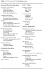
4.6 PLASMA PROCESSING SYSTEMS A good plasma system must first be a good vacuum system since c ontaminants will be activated in the plasm a. In comparison to vacuum processing systems the plasma processing systems are complicated by: • High gas loads from the introduction of processing gases • Often a reduced pumping speed (gas throughput) in the deposition chamber • Potentially explosive or flammable gases are used in some plasma-based processes In many cases the generalized vacuum processing system shown in Fig. 3-8 may be used with a plasma in the processing chamber if the pumping system and fixturing is designed appropriately. Flow control for establishing the gas pressure needed to form a plasma, can be done by partially closing (throttling) the high vacuum valve , by using a variable conductance valve in series with the high vacuum valve or by the addition of the optional gas flow path as indicated. The electrode for forming the plasma (“glow bar”) is positioned so as to extend into as large a region of the chamber as possible. In plasma processing, the deposition conditions differ greatly depending on whether the substrate is placed on an active electrode , in the plasma generation region or in a “remote position” where the plasma afterglow is found. Plasma-based processes may either be clean or “dirty .” Sputter deposition and ion plating are generally relatively clean processes while plasma etching and plasma-enhanced CVD are dirty processes. The main equipment-related problems in plasma-based PVD processing are: • Production of a plasma having desirable and uniform properties in critical regions of the processing volume • Control of the mass flow rate and composition of the gases and vapors introduced into the system • Removal of unused processing gases , reaction products and contaminant gases and vapors from the processing volume • Prevention of charge buildup and arcing • Corrosion if corrosive gases or vapors are used in the processing
1.1 SURFACE ENGINEERING Surface engineering involves changing the properties of the surface and near-surface region in a desirable way. Surface engineering can involve an overlay process or a surface modification process . In overlay processes a material is added to the surface and the underlying material (substrate) is covered and not detectable on the surface. A surface modification process changes the properties of the surface but the substrate material is still present on the surface. For example, in aluminum anodization, oxygen reacts with the anodic aluminum electrode of an electrolysis cell to produce a thick oxide layer on the aluminum surface. Table 1-1 shows a number of overlay and surface modification processes that can be used for surface engineering. Each process has its advantages, disadvantages and applications . In some cases surface modification processes can be used to modify the substrate surface prior to depositing a film or coating. For example a steel surface can be hardened by plasma nitriding (ionitriding) prior to the deposition of a hard coating by a PVD process. In other cases , a surface modification process can be used to change the properties of an overlay coating. For example, a sputter-deposited coating on an aircraft turbine blade can be shot peened to densify the coating and place it into compressive stress. An atomistic film deposition process is one in which the overlay material is deposited atom-by-atom. The resulting film can range from single crystal to amorphous, fully dense to less than fully dense, pure to impure, and thin to thick. Generally the term “thin film” is applied to layers which have thicknesses on the order of several microns or less (1 micron = 10 -6 meters) and may be as thin as a few atomic layers. Often the properties of thin films are affected by the properties of the underlying material (substrate) and can vary through the thickness of the film . Thicker layers are generally called coatings . Atomistic deposition process can be done in a vacuum, plasma, gaseous, or electrolytic environment.
Classical Paper List on Machine Learning and Natural Language Processing from Zhiyuan Liu Hidden Markov Models Rabiner, L. A Tutorial on Hidden Markov Models and Selected Applications in Speech Recognition. (Proceedings of the IEEE 1989) Freitag and McCallum, 2000, Information Extraction with HMM Structures Learned by Stochastic Optimization, (AAAI'00) Maximum Entropy Adwait R. A Maximum Entropy Model for POS tagging, (1994) A. Berger, S. Della Pietra, and V. Della Pietra. A maximum entropy approach to natural language processing. (CL'1996) A. Ratnaparkhi. Maximum Entropy Models for Natural Language Ambiguity Resolution. PhD thesis, University of Pennsylvania, 1998. Hai Leong Chieu, 2002. A Maximum Entropy Approach to Information Extraction from Semi-Structured and Free Text, (AAAI'02) MEMM McCallum et al., 2000, Maximum Entropy Markov Models for Information Extraction and Segmentation, (ICML'00) Punyakanok and Roth, 2001, The Use of Classifiers in Sequential Inference. (NIPS'01) Perceptron McCallum, 2002 Discriminative Training Methods for Hidden Markov Models: Theory and Experiments with Perceptron Algorithms (EMNLP'02) Y. Li, K. Bontcheva, and H. Cunningham. Using Uneven-Margins SVM and Perceptron for Information Extraction. (CoNLL'05) SVM Z. Zhang. Weakly-Supervised Relation Classification for Information Extraction (CIKM'04) H. Han et al. Automatic Document Metadata Extraction using Support Vector Machines (JCDL'03) Aidan Finn and Nicholas Kushmerick. Multi-level Boundary Classification for Information Extraction (ECML'2004) Yves Grandvalet, Johnny Marià , A Probabilistic Interpretation of SVMs with an Application to Unbalanced Classification. (NIPS' 05) CRFs J. Lafferty et al. Conditional Random Fields: Probabilistic Models for Segmenting and Labeling Sequence Data. (ICML'01) Hanna Wallach. Efficient Training of Conditional Random Fields. MS Thesis 2002 Taskar, B., Abbeel, P., and Koller, D. Discriminative probabilistic models for relational data. (UAI'02) Fei Sha and Fernando Pereira. Shallow Parsing with Conditional Random Fields. (HLT/NAACL 2003) B. Taskar, C. Guestrin, and D. Koller. Max-margin markov networks. (NIPS'2003) S. Sarawagi and W. W. Cohen. Semi-Markov Conditional Random Fields for Information Extraction (NIPS'04) Brian Roark et al. Discriminative Language Modeling with Conditional Random Fields and the Perceptron Algorithm (ACL'2004) H. M. Wallach. Conditional Random Fields: An Introduction (2004) Kristjansson, T.; Culotta, A.; Viola, P.; and McCallum, A. Interactive Information Extraction with Constrained Conditional Random Fields. (AAAI'2004) Sunita Sarawagi and William W. Cohen. Semi-Markov Conditional Random Fields for Information Extraction. (NIPS'2004) John Lafferty, Xiaojin Zhu, and Yan Liu. Kernel Conditional Random Fields: Representation and Clique Selection. (ICML'2004) Topic Models Thomas Hofmann. Probabilistic Latent Semantic Indexing. (SIGIR'1999). David Blei, et al. Latent Dirichlet allocation. (JMLR'2003). Thomas L. Griffiths, Mark Steyvers. Finding Scientific Topics. (PNAS'2004). POS Tagging J. Kupiec. Robust part-of-speech tagging using a hidden Markov model. (Computer Speech and Language'1992) Hinrich Schutze and Yoram Singer. Part-of-Speech Tagging using a Variable Memory Markov Model. (ACL'1994) Adwait Ratnaparkhi. A maximum entropy model for part-of-speech tagging. (EMNLP'1996) Noun Phrase Extraction E. Xun, C. Huang, and M. Zhou. A Unified Statistical Model for the Identification of English baseNP. (ACL'00) Named Entity Recognition Andrew McCallum and Wei Li. Early Results for Named Entity Recognition with Conditional Random Fields, Feature Induction and Web-enhanced Lexicons. (CoNLL'2003). Moshe Fresko et al. A Hybrid Approach to NER by MEMM and Manual Rules, (CIKM'2005). Chinese Word Segmentation Fuchun Peng et al. Chinese Segmentation and New Word Detection using Conditional Random Fields, COLING 2004. Document Data Extraction Andrew McCallum, Dayne Freitag, and Fernando Pereira. Maximum entropy Markov models for information extraction and segmentation. (ICML'2000). David Pinto, Andrew McCallum, etc. Table Extraction Using Conditional Random Fields. SIGIR 2003. Fuchun Peng and Andrew McCallum. Accurate Information Extraction from Research Papers using Conditional Random Fields. (HLT-NAACL'2004) V. Carvalho, W. Cohen. Learning to Extract Signature and Reply Lines from Email. In Proc. of Conference on Email and Spam (CEAS'04) 2004. Jie Tang, Hang Li, Yunbo Cao, and Zhaohui Tang, Email Data Cleaning, SIGKDD'05 P. Viola, and M. Narasimhan. Learning to Extract Information from Semi-structured Text using a Discriminative Context Free Grammar. (SIGIR'05) Yunhua Hu, Hang Li, Yunbo Cao, Dmitriy Meyerzon, Li Teng, and Qinghua Zheng, Automatic Extraction of Titles from General Documents using Machine Learning, Information Processing and Management, 2006 Web Data Extraction Ariadna Quattoni, Michael Collins, and Trevor Darrell. Conditional Random Fields for Object Recognition. (NIPS'2004) Yunhua Hu, Guomao Xin, Ruihua Song, Guoping Hu, Shuming Shi, Yunbo Cao, and Hang Li, Title Extraction from Bodies of HTML Documents and Its Application to Web Page Retrieval, (SIGIR'05) Jun Zhu et al. Mutual Enhancement of Record Detection and Attribute Labeling in Web Data Extraction. (SIGKDD 2006) Event Extraction Kiyotaka Uchimoto, Qing Ma, Masaki Murata, Hiromi Ozaku, and Hitoshi Isahara. Named Entity Extraction Based on A Maximum Entropy Model and Transformation Rules. (ACL'2000) GuoDong Zhou and Jian Su. Named Entity Recognition using an HMM-based Chunk Tagger (ACL'2002) Hai Leong Chieu and Hwee Tou Ng. Named Entity Recognition: A Maximum Entropy Approach Using Global Information. (COLING'2002) Wei Li and Andrew McCallum. Rapid development of Hindi named entity recognition using conditional random fields and feature induction. ACM Trans. Asian Lang. Inf. Process. 2003 Question Answering Rohini K. Srihari and Wei Li. Information Extraction Supported Question Answering. (TREC'1999) Eric Nyberg et al. The JAVELIN Question-Answering System at TREC 2003: A Multi-Strategh Approach with Dynamic Planning. (TREC'2003) Natural Language Parsing Leonid Peshkin and Avi Pfeffer. Bayesian Information Extraction Network. (IJCAI'2003) Joon-Ho Lim et al. Semantic Role Labeling using Maximum Entropy Model. (CoNLL'2004) Trevor Cohn et al. Semantic Role Labeling with Tree Conditional Random Fields. (CoNLL'2005) Kristina toutanova, Aria Haghighi, and Christopher D. Manning. Joint Learning Improves Semantic Role Labeling. (ACL'2005) Shallow parsing Ferran Pla, Antonio Molina, and Natividad Prieto. Improving text chunking by means of lexical-contextual information in statistical language models. (CoNLL'2000) GuoDong Zhou, Jian Su, and TongGuan Tey. Hybrid text chunking. (CoNLL'2000) Fei Sha and Fernando Pereira. Shallow Parsing with Conditional Random Fields. (HLT-NAACL'2003) Acknowledgement Dr. Hang Li , for original paper list.
Please read carefully!! To submit a new manuscript, click on the blue star in the right column. Clicking on the various manuscript status links under My Manuscripts will display a list of all the manuscripts in that status at the bottom of the screen. To continue a submission already in progress, click the Continue Submission link in the Unsubmitted Manuscripts list. To submit a revision , click the Manuscripts with Decisions link in the left navigation. When you click on Create a Revision, your new submission record will be pre-populated with information from your original submission. Please update the manuscript record to reflect the characteristics of your revision. Please remember to include in a new manuscript submission: The required single-column double-spaced (1-column) version of the manuscript which may not exceed 30 pages for regular paper, 12 pages for correspondence and 3 pages for comment correspondence. The required double-column single-spaced (2-column) version of the manuscript which shall be no more than 10 pages for regular paper, or 6 pages for correspondence. Manuscripts that exceed these limits will incur mandatory overlength page charges. VERY IMPORTANT NOTE: In accordance with the Societys Information for Authors, all Signal Processing Society Journals do not accept the IEEE Electronic Copyright Form with electronic signature. When you are redirected to the IEEE Electronic Copyright Form wizard at https://ecopyright.ieee.org/ECTT/login.jsp?referer=blank at the end of your submission, please simply exit it and submit your hand signed form to the SPS office either by fax or e-mail. You may also upload the form as a Supporting Document when submitting your manuscript files to the MC system. The properly executed and signed IEEE Copyright Form. The IEEE Copyright Form is available online at http://www.ieee.org/web/publications/rights/copyrightmain.html. The form can be uploaded on MC as supporting document or print the form, complete it (PAPER# ON TOP, paper title, author names, publication title, handwritten signature and date) and send it by fax to the IEEE Signal Processing Society Publications Office at +1 732 235 1627/ +1 732 562 8905, or e-mail a scanned version to z.kowalski@ieee.org. Please note that your manuscript will not be processed for review if a properly executed copyright form is not received by the publications office. Failure to comply with this requirement will result in the immediate rejection of the manuscript. Please refer to Instructions Forms for more detailed information: Information for Authors: http://ieeexplore.ieee.org/stamp/stamp.jsp?arnumber=04799354 Author Guide : http://mcv3help.manuscriptcentral.com/tutorials/Author.pdf The Online Training Documentation Resources : (here you will find Online Users Guides and Quick Start Guides, such as the Editor Guide, Reviewer Guide, Author Guide)
 标签: processing