等高线图是另一类重要的 3D 绘图方式。为了说明 gnuplot 里面等高线图的绘制方法,我们使用下面这个数据文件作为例子: surface.dat 首先绘制普通曲面图: gnuplot set hidden3d gnuplot splot "surface.dat" with lines 下面加上等高线: gnuplot set contour base gnuplot splot "surface.dat" with lines title "" set contour 命令之后除了 base 参数外,还可以使用 surface 或 both 参数,分别表示等高线画在底面、曲面或者两者都画。这里设置了一个空的 title ,是为了在图例中不要显示文件名,以免和等高线的图例混淆。 如果我们想在平面中显示等高线,可以使用下列命令: gnuplot unset surface gnuplot set view map gnuplot set size square gnuplot replot 如果我们想在之前提到过的 pm3d 图上显示等高线,可以这样做: gnuplot set pm3d at b gnuplot set key at screen 0.8,0.8 gnuplot replot 这里我们把图例的位置做了调整,因为默认图例是在图像里面的,这样可能影响我们的图像显示。 最后,我们谈谈怎样手动设置等高线数值和间距。等高线的数值间隔参数设置命令是 set cntrparam levels 。默认情况下,gnuplot 自动设置等高线数值。如果要进行手动设置,有两种方法: incremental start,incr,end 设置起始值以及间隔大小,这种方法适用于等间隔的等高线; discrete z1,z2,z3,… 分别设置各个等高线数值,这种方法适用于间隔不等的等高线。 例子: gnuplot set cntrparam levels incremental -2,0.5,2 gnuplot replot
Error bar 是在图像上表现数据误差范围的一种方式。对于含有误差项的数据,除了通常的 x 轴和 y 轴两列数据外,我们还需要有额外的误差数据列。 拿 x 数据列举例,如果误差用标准差 σ x 来表示,那么数据取值范围可以表示为 ,这时候只要增加一列误差项就行了,所以一共需要 3 列数据。如果误差用最小值 x min 和最大值 x max 来表示,那么数据取值范围可以表示为 ,这时候需要增加两列误差项,所以一共需要 4 列数据。对于 y 数据误差,表达方法和 x 类似。如果同时包含 x 和 y 误差,就需要把两者结合起来。 在 gnuplot 里,error bar 的基本使用方法是: plot "数据文件名" using using参数 with xerrorbars | yerrorbars | xyerrorbars using 命令在之前的“ 多组数据绘图 ”博文里已经介绍过,目的是选择哪些列数据进行绘图,数据列数必须和后面选择的绘图方式对应。 with 命令后面跟的是绘图方式,选择用 xerrorbars , yerrorbars ,还是 xyerrorbars 。根据不同绘图方式,所需数据列数分别为: xerrorbars 3 列: x y σ x 4 列: x y x min x max yerrorbars 3 列: x y σ y 4 列: x y y min y max xyerrorbars 4 列: x y σ x σ y 6 列: x y x min x max y min y max 下面我们举一个例子,这是一个测量在液体中聚焦的脉冲激光在焦点处产生气泡几率的实验,数据文件(probability.dat)如下: ### 文件开始 ### # Ave Energy Probability Min Energy Max Energy Energy SD # (micro J) (%) (micro J) (micro J) (micro J) # ======================================================================= 9.08 0 8.96 9.15 0.06 10.00 2 9.91 10.08 0.05 10.52 3 10.41 10.60 0.06 11.03 10 10.90 11.11 0.06 11.52 25 11.38 11.62 0.07 12.03 57 11.90 12.13 0.07 12.52 88 12.38 12.64 0.08 13.01 93 12.86 13.09 0.07 13.51 100 13.38 13.61 0.08 14.52 100 14.38 14.67 0.08 ### 文件结束 ### x 轴数据为激光能量,y 轴数据为气泡产生几率,这里只有 x 误差,并且同时包含了最小最大值和标准差。我们现在用最小最大值画图: gnuplot set xrange gnuplot set yrange gnuplot unset key gnuplot set xlabel "Laser Pulse Energy (μJ)" gnuplot set ylabel "Bubble Formation Probability (%)" gnuplot plot "probability.dat" using 1:2:3:4 with xerrorbars 如果既要画 error bar,又要连线,可以把上述命令中的 errorbars 换为 errorlines : gnuplot plot "probability.dat" using 1:2:3:4 with xerrorlines
gnuplot 也能画参数方程。首先设置参数方程环境: gnuplot set parametric 然后我们会看见返回信息: dummy variable is t for curves, u/v for surfaces 和极坐标类似,参数方程的自变量也是 t 。后面的 u/v 是用于 3D 绘图的参数方程自变量,我们目前暂时不管它。 对于参数方程 x = f(t), y = g(t) ,绘图命令为 plot f(t),g(t) 下面我们看一个例子,这是一个李萨如(Lissajous)曲线: gnuplot set parametric gnuplot set xrange gnuplot set yrange gnuplot set trange gnuplot set samples 1000 gnuplot set size square gnuplot unset key gnuplot plot sin(3*t),sin(4*t) lw 2
在同一图像中包含多组数据或函数时,图例是必要的。我们这一次谈一谈图例的微调。 这次来画前 3 阶的第一类贝塞尔函数 J n (x) 。在 gnuplot 里,0 阶和 1 阶贝塞尔函数已经定义了,分别为 besj0(x) 和 besj1(x) ,而 2 阶贝塞尔函数可以通过递推关系构造出来。下面是例子: gnuplot set term wxt enhanced gnuplot besj2(x) = besj1(x)*2/x - besj0(x) gnuplot set xrange gnuplot set xtics 2 gnuplot set xlabel "X" gnuplot set ylabel "Y" gnuplot set title "Bessel Functions of the First Kind" gnuplot set grid gnuplot set style line 1 lw 2 lc rgb "#F62217" gnuplot set style line 2 lw 2 lc rgb "#D4A017" gnuplot set style line 3 lw 2 lc rgb "#2B60DE" gnuplot plot besj0(x) ls 1 t "J_0(x)", besj1(x) ls 2 t "J_1(x)", besj2(x) ls 3 t "J_2(x)" 之前我们讲过, plot 命令后面可以跟随一些参数(例如 linewidth , linecolor 等)来改变点线风格。在上面的例子中,我们把这些参数单独拿出来放到了 set style 命令里,定义了三个 linestyle ,然后在 plot 命令里再调用这些 linestyle 。这样子做和我们之前的做法效果上没什么不同,唯一的区别是让 plot 命令短了一些。另外,改变风格可能容易一点。 上面是默认的图例,下面让我们进行微调。 为图例加上边框 gnuplot set key box gnuplot replot 改变图例显示位置 gnuplot set key center at 10,0.7 gnuplot replot 把图例的 title 和图线示例调换位置 gnuplot set key reverse gnuplot replot 调整图例边框宽度 width (或高度 height ) gnuplot set key width 1 gnuplot replot 调整 title 文字对齐方式( Left 或者 Right ,注意首字母大写) gnuplot set key Left gnuplot replot 调整图例行间隔 gnuplot set key spacing 1.2 gnuplot replot 调整图线示例长度 gnuplot set key samplen 2 gnuplot replot 这些并不是 set key 的全部参数。在 gnuplot 里,如果想深入了解任何命令的详细用法,不要忘记使用 help 命令。
我们现在所有绘图的坐标刻度均标在图像边框上,无论上下左右。这样做的好处是函数或数据图线清楚,不会和坐标标注混在一起。其实,我们小时候数学课上最早学习坐标系的时候,都是让 X 轴和 Y 轴正交于原点,而刻度标注在坐标轴上。这样的图像在定性表现函数关系,尤其有一定对称性的函数关系时,比较一目了然。 让我们来看看怎样用 gnuplot 得到这样的效果。 用 unset border 命令把边框去掉; 用 set zeroaxis 命令画出正交于原点的坐标轴; 在设定坐标刻度时加上 axis 参数,这样刻度会出现在坐标轴上面,而不是边框上。 为了避免审美疲劳,这次我们拿高斯函数举个例子: gnuplot set term wxt enhanced font "Times New Roman,16" gnuplot gauss(x) = exp(-pi*x*x) gnuplot set title "函数 e^{-πx^2}" gnuplot set samples 500 gnuplot set xrange gnuplot set yrange gnuplot unset key gnuplot unset border gnuplot set zeroaxis lt -1 lw 2 gnuplot set xtics axis -2,1,2 gnuplot set ytics axis 0,1,1 gnuplot plot gauss(x) lw 3 例子中的参数前面都介绍过,如果不记得了,可以复习一下“ 坐标取值范围及刻度 ”和“ 点线风格 ”等章节。这里的图像已经很像模像样了,除了标签位置还不那么理想,而且坐标轴没有箭头。幸好,我们上一讲刚刚谈到过箭头,下面来试试做一下微调: gnuplot set title "函数 e^{-πx^2}" offset 12,-5 gnuplot set xtics axis -2,1,2 offset 0.4,0 gnuplot set ytics axis 0,1,1 offset 0,0.4 gnuplot set arrow 1 from 2,0 to 3.2,0 filled size 0.2,15,60 lw 2 gnuplot set arrow 2 from 0,1 to 0,1.22 filled size 0.2,15,60 lw 2 gnuplot set rmargin 4 gnuplot set label 1 "X" at 3.0,-0.1 gnuplot set label 2 "Y" at -0.3,1.2 gnuplot replot 这里有几个命令同时用到了新的参数: offset 。它的作用就是把命令里提到的标签文字平移一段距离。在这里, offset 默认的坐标系统是 character 。我们慢慢会体会到这种做法的好处,它使得我们很多时候改变字体大小,而不必重新设置 offset 。 另外, set rmargin 命令用于设置图像右边空白宽度,单位也是 character 。一般情况下,四边空白宽度都是自动设置的。现在我们在右边增加了箭头,而绘图显示区域不会因此自动扩大,这样会导致箭头无法完整显示,所以要手动改一下设置。相应的,上、左、下边的空白宽度,分别由 tmargin , lmargin , bmargin 参数控制。
我们现在知道了 gnuplot 有第一( first )和第二( second )两套坐标系统,但是 gnuplot 的坐标系统还不止于此。除此之外,它还有 graph , screen 和 character 三套坐标系统。 graph 和 screen 都是归一化的坐标系统。 graph 以坐标轴包围区域为界,左下角为 0,0 ,右上角为 1,1 ; screen 以整个图片区域为界,左下角为 0,0 ,右上角为 1,1 。 character 顾名思义,是以字符大小为单位长度的坐标系统,因此它的单位长度依赖于字体大小。它的原点位置和 screen 相同。 下面我们结合 label 命令来了解一下这几个坐标系统。我们之前讲过 xlabel 和 ylabel 。而这里的 label 命令,是在图中任何地方插入文字标签。还是来看例子: gnuplot sinc(x) = sin(pi*x)/(pi*x) gnuplot set xlabel "X" gnuplot set ylabel "Y" gnuplot unset key gnuplot set samples 500 gnuplot set xrange gnuplot set xtics 1 gnuplot set x2range gnuplot set x2tics 1 gnuplot set y2range gnuplot set y2tics 1 gnuplot set grid gnuplot set label 1 "Hello first" at 2,0.5 gnuplot set label 2 "Hello second" at second 2,0.5 gnuplot set label 3 "Hello graph" at graph 0.2,0.5 gnuplot set label 4 "Hello screen" at screen 0.2,0.5 gnuplot set label 5 "Hello character" at character 10,5 gnuplot plot sinc(x) 这里我们画一个 sinc 函数图像。为了说明问题,我们把第二坐标系也都标示了出来,虽然函数图像并没有用到第二坐标。其他命令前面都讲过了,这里只看五个 set label 命令。 set label 之后紧跟的那个整数,就是一个标识符,用以区别各个 label ,可以随便选个整数。在字符串之后, at 参数指定标签坐标。默认为 first 坐标系统,也可以使用其它坐标系统。下面是生成的图片: 为了帮助大家理解,我们把 graph 和 screen 各自的坐标区域分别用绿色和橙色表示了出来。 标签文字的默认对齐方式为居左,也就是指定的坐标位置在文字的左边。我们也可以在 label 命令里选择其他对齐方式。除此之外,我们还可以在 label 命令里指定文字颜色,旋转文字,或者在指定坐标位置处加一个点。下面例子中的每个参数不必一一解释了,因为和我们前面接触过的命令都是一致的: gnuplot set label 1 "Hello red left" at 2,0.4 left textcolor rgb "#FF0000" gnuplot set label 2 "Hello green center" at 2,0.5 center textcolor rgb "#00FF00" gnuplot set label 3 "Hello blue right" at 2,0.6 right textcolor rgb "#0000FF" gnuplot set label 4 "Hello rotate" at -2,0.4 rotate by 45 gnuplot set label 5 "Hello point" at -3,0.2 point pt 7 lc rgb "#FF9900" gnuplot replot
 标签: Gnuplot