source:http://statistics.about.com/od/ProbHelpandTutorials/a/How-Are-Odds-Related-To-Probability.htm Many times the odds of an event occurring are posted. One might say that a particular sports team is a 2:1 favorite to win the big game. This may also be stated that the odds in favor of our team winning are two to one. What many people do not realize is that these odds are really just a restatement of the probability of an event. Notation for Odds We express our odds as a ratio of one number to another. Typically we read the ratio A : B as A to B . Each number of these ratios can be multiplied by the same number. So the odds 1:2 is equivalent to saying 5:10. Probability to Odds Probability can be carefully defined using set theory and a few axioms , but the basic idea is that probability uses a real number between zero and one to measure the likelihood of an event occurring. There are a variety of ways to think about how to compute this number. One way is to think about performing an experiment several times. We count the number of times that the experiment is successful and then divide this number by the total number of trials of the experiment. If we have A successes out of a total of N trials, then the probability of a success is A / N . But if we instead consider the number of successes versus the number of failures, we are now calculating the odds in favor of an event. If there were N trials and A successes, then there were N - A = B failures. So the odds in favor are A to B . We can also express this as A : B . An Example of Probability to Odds In the past five seasons, crosstown football rivals the Quakers and the Comets have played each other with the Comets winning twice and the Quakers winning three times. On the basis of these outcomes, we can calculate the probability the Quakers win and the odds in favor of their winning. There were a total of three wins out of five, so the probability of winning this year is 3/5 = 0.6 = 60%. Expressed in terms of odds, we have that there were three wins for the Quakers and two losses, so the odds in favor of them winning are 3:2. Odds to Probability The calculation can go the other way. We can start with odds for an event and then derive it’s probability. If we know that the odds in favor of an event are A to B , then this means that there were A successes for A + B trials. This means that the probability of the event is A /( A + B ). An Example of Odds to Probability A clinical trial reports that a new drug has odds of 5 to 1 in favor of curing a disease. What is the probability that this drug will cure the disease? Here we say that for every five times that the drug cures a patient, there is one time where it does not. This gives a probability of 5/6 that the drug will cure a given patient. Why Use Odds? Probability is nice, and gets the job done, so why do we have an alternate way to express it? Odds can be helpful when we want to compare how much larger one probability is relative to another. An event with probability 75% has odds of 75 to 25. We can simplify this to 3 to 1. This means that the event is three times more likely to occur than not occur. another reference:http://pages.uoregon.edu/aarong/teaching/G4075_Outline/node15.html
(For new reader and those who request 好友请求, please read my 公告栏 first) Probability and Stochastic Process Tutorial (1) Probability is often characterized as “ a precise way to deal with our ignorance or uncertainty ”. Everyone has an intuitive understanding of the question “what are the chance of (something happening)?”. Stochastic process is then dealing with probabilities over time (or over some independent and indexed variable such as distance). There exist a number of excellent or classic textbooks on probability and stochastic processes. It is one of my favorite oral examine question which I always tell student beforehand to prepare as well as in my opinion the most useful tools of an applied mathematician and/or engineer. http://blog.sciencenet.cn/home.php?mod=spaceuid=1565do=blogid=13708 and http://blog.sciencenet.cn/home.php?mod=spaceuid=1565do=blogid=656455 Yet in my experience it is also one of the most confusing subjects for many students to learn. Why? In this series of blog articles (of which this is the first) I shall try to explain the subject in my own way and my experience in learning the subject. It is NOT my intention to replace the excellent textbooks . The main purpose of these articles, I hope, is that by reading the articles will make the subject matter more approachable and less imposing. They are NOT meant toreplace the many excellent textbook on the subject . I write this article not in the rigorous style required for a scholastic textbook but more in the spirit of a teacher who is engaged in a face-to-face session with a student. It will be highly informal but will make the big picture come across easier. Hopefully, it will even make it possible to read and gain insight to textbooks and articles written in measure-theoretic language. My approach will be strictly from a user point of view requiring nothing beyond freshman calculus and ability to visualize n-dimensional space as a natural generalization of our familiar 3-D space. So here goes . . . Let us start by making one simplifying assumption which for people interested in practical application is not at all important or restrictive. This is the Finiteness Assumption (FA) – We assume there is no INFINITLY large number, i.e., no infinity but there can be very large numbers, e.g. 10^100 (a number estimated to be larger than the total number of atoms in the universe.) If one deals only with real computation on digital computers, this assumption is automatically satisfied. By making this assumption we assume away all the measure-theoretic terminologies that populate theoretical probability literature and confuse the uninitiated. With the FA assumption we now define what is a random variable. Random Variable (r.v.) – a random variable is a variable that may take on any number of finite values when sampled (i.e. looked at). We characterize ar.v. by specifying its histogram. A histogram spells out which sampled values in a range of values the r.v. may take on what percentage of the time. Fig. 1 it a typical histogram. It is actually a histogram of a random variable which is the readership (or hits) of my blog articles for the pastfour years. Fig. 1 histogram of readership of my blog articles (2009-2013): x-axis is #of hits, y-axis is #of article in this hit range Note each bar of the histogram is expressed as a percentage so that the total sum of bars adds up to one or 100%, i.e., with probability one (for sure) the r.v. takes on values somewhere in the total range. While the range of values this r.v. may take on is finite by virtue of assumption FA , to completely specify a r.v. still can take a great deal of data. (In fact, it took me about 3 hours to collect data and make this graph which is why I did not compile the data for all 5+ year of my blog life) This is inconvenient in computation. To simplify the description (specification) we develop two common rough characterizations. The Mean of a r.v. – Intuitively, if you imagine a cardboard cutout of the shape of the histogram, then the value along the x-axis at which a knife edge placed perpendicular to the x-axis that will balance this cardboard shape is the mean of this r.v..Mathematically, it is simply the average of the value of hits for each article, the ScienceNet in fact compute this value for all bloggers and displays the top-100 bloggers. My own current average happens to be 4130 per article and ranks 26th on the list. Variance of ar.v. - This is a measure of the spread of the histogram. A small variance roughly mean the histogram is mostly spread over a small range of numbers around its mean and vice versa for a large variance. It is a measure of the variability of the values of the r.v.. In stock marketterminology, the b of a stock is simply the variance of the daily value of the stock and a measure of its volatility. Mathematically variance is called the second central moments of the histogram Now we can develop further rough characterization of the histogram by defining what are called its higher central moments, such as skewness of the histogram, which is the third central moment . But in practice such higher moment are rarely needed nor data on these moments often available. So much for a single r.v.. But we often have to deals with more than one random variable. Let us consider two r.v.s, x and y. Now the histogram of the random variables x-y becomes a 3D object. Graphically it looks like a multi-peak terrain map (think of Quilin in the Kwangxi province of south China or the skyscrapers of the Manhattan island of NY). But here a new concept intrudes. It is called “ joint probability ” or “ correlation/covariance (in case of an approximate specification)” between the r.v.s x and y. It captures relationship, if any, between the r.v.s. We are all familiar with notion that smart parents tends to produce smart children. If we represent the intelligence of parents as r.v. x and that of the child is .r.v y, then mathematically we say y is positively correlated with x. If we look down on the 3D histogram of x and y, then we shall see the peaks scatter along a northeast to southwest direction as illustrated in Fig.2 FIg.2 bird’s eye view of 3D histogram with correlation In other words, knowing the value of y will give a different idea about the probable value of x. More generally we say x and y are NOT independent but correlated . Mathematically we denote the joint probability p(x,y) (i.e., the histogram) as a general 3D function. We also define conditional probability of x given the value of y as p(x/y) p(x,y)/p(y) or p(y/x) p(x,y)/p(x) Where p(y) and p(x) , called marginally probability of y and x respectively are simply the resultant 2D histograms when we collapse the 3D histogram onto the y or x axis respectively. Graphically, the conditional probability p(x/y) is simply the 2D histogram one sees if we take a cross sectional view of the 3D histogram at the particular value of y. Mathematically we need to divide p(x,y) by p(y) to normalize the values so that p(x/y) will still have area equal to one (100%) satisfying the definition of a histogram. Now it is possible that the bird’s eye view of the 3D histogram is a rectangle (vs. the view of Fig. 2). In other word p(x/y)=p(x) no matter which value of y we choose. In this case, by definition of p(x/y), we have p(x,y)=p(y)p(x). We say the r.v.s x and y are independent . Intuitively this satisfies the notion that knowing y does not tell us anything new about the probable values of x and vice versa about y when knowing x. Computationally, this simplifies a function of 2 variables into product of single variable functions, a great computational simplification when n random variables are involved. To roughly characterize the two generalr.v.s we have a mean vector and a 2x2 covariance matrix with diagonal element the variance of x and y and the symmetrical covariance in the off-diagonal position s x 2 s xy s yx s y 2 To summarize. We have so far introduced concepts 1. Random variable characterized by histograms 2. Rough characterization of histograms by mean and variance 3. Joint probability (3D histogram) of two r.v.s 4. Independence and conditional probability 5. Covariance matrix Now suppose we have n r.v.s instead of two, everything I said about the two r.v.s apply. We merely have to change 2D and 3D to n and n+1 dimensions. The mean of n r.v.s becomes a n-vector and the covariance matrix is a nxn matrix. In your mind’s eye you can visualize everything in n dimension the same way as Fig.1 and 2. The joint probability (histogram) p(x 1 , x 2 , . . . , x) is a n variable function. And if the n variables are independent from each other, we write p(x 1 , x 2 , . . . , x n )=p(x 1 )p(x 2 ). . . p(x n ). No new concepts are involved. Concept-wise, believe it or not, these in my opinion are all you need to know about probability and stochastic processes to function in the engineering world even if your interest is academic and theoretical . In my 46 years of active research and engineering consulting in stochastic control and optimization, I never had to go beyond the knowledge described above. The following articles will simply illustrate and explain how to apply these ideas to more practical uses. Computationally, because of exponential growth, to deal with arbitrary n-variable function is impossible. http://blog.sciencenet.cn/blog-1565-26889.html . Data-wise, it also involve astronomically large amount of data. To simplify notations at least theoretically, we make a continuous approximation of these discrete data and introduce continuous variables and functions. To emphasize, for our purpose, this is only a convenient approximation and simplification. No new ideas are involved. This will be the content of next article. Beyond introducing continuous variables, we also need to develop carious special cases of joint probability structures to simplify description and calculations, subsequent articles will address these issues. Once again, let me emphasize that from my view point these simplifications and special cases are need for computational feasibility and practicality. Nothing conceptually new is involved.
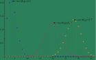
A hypergeometric experiment possesses the following properties: 1. A population contains a finite number $N$ of elements that possess one of two characteristics, say, red and black. 2. $r$ of the elements are red and the others black. 3. A sample of n elements is randomly selected from the population. 4. The random variable of interest is Y , the number of red elements in the sample. Definition: A random variable Y is said to have a hypergeometric probability distribution if and only if $$p(y) = \frac{{\left( {\begin{array}{*{20}{c}} r\\ y \end{array}} \right)\left( {\begin{array}{*{20}{c}} {N - r}\\ {n - y} \end{array}} \right)}}{{\left( {\begin{array}{*{20}{c}} N\\ n \end{array}} \right)}}$$ where $y$ is an integer 0, 1, 2, ..., n, subject to the restrictions $y \le r$ and $n-y \le N-r$. You can use the following Mathematica command to obtain the probability PDF , y] // TraditionalForm Relative Mathematica Function HypergeometricDistribution Gives the distribution of the number of red elements in n draws from a population of sizeN containingr red elements. Examples: A := HypergeometricDistribution ; a1 = {Arrowheads , Arrow , 5]}}]}; t1 = Text ",r=50,N=100", Medium], {10, 0.25}, {-1, 0}]; a2 = {Arrowheads , Arrow , 10]}}]}; t2 = Text ",r=50,N=100", Medium], {12, 0.23}, {-1, 0}]; a3 = {Arrowheads , Arrow , 25]}}]}; t3 = Text ",r=50,N=100", Medium], {25, 0.20}, {0, -1}]; epilog = {a1, t1, a2, t2, a3, t3}; DiscretePlot , k], {n, {10, 20, 50}}], {k, 0, 32}, PlotRange - All, PlotMarkers - Automatic, Epilog - epilog, Background - RGBColor ] Expection and Variance: If Y is a random variable with a hypergeometric distribution,then, $$E(Y) = \frac{{nr}}{N}\;\;\;{\rm{and}}\;\;\;V(Y) = n\left( {\frac{r}{N}} \right)\left( {\frac{{N - r}}{N}} \right)\left( {\frac{{N - n}}{{N - 1}}} \right).$$ You can use the following Mathematica command to obtain these results Expectation HypergeometricDistribution ] or Mean ] Variance ] Property: For a fixed fraction $p = \frac{r}{N}$, the hypergeometric probability function converges to the binomial probability function as $N$ becomes large and $n$ is relatively small. $$\mathop {\lim }\limits_{N \to \infty } \frac{{\left( {\begin{array}{*{20}{c}} r\\ y \end{array}} \right)\left( {\begin{array}{*{20}{c}} {N - r}\\ {N - y} \end{array}} \right)}}{{\left( {\begin{array}{*{20}{c}} N\\ n \end{array}} \right)}} = \left( {\begin{array}{*{20}{c}} n\\ y \end{array}} \right){p^y}{\left( {1 - p} \right)^{n - y}}.$$
A Negative Binomial experiment possesses the following properties: 1. The experiment consists of aseries of identical trials. 2. Each trial results in one of two outcomes: success, S, or failure, F. 3. The probability of success on a single trial is equal to some value p and remains the same from trial totrial. The probability of a failure is equal to q = (1 − p). 4. The trials are independent. 5. The random variable of interest is Y , the number of failures before n successes occur. Definition: A random variable Y is said to have anegative binomialprobability distribution if and only if $$p(y) = \left( {\begin{array}{*{20}{c}} {n + y - 1}\\ {n - 1} \end{array}} \right){p^n}{(1 - p)^y},\;\;\;\;y = 0,\;1,\;...,\;\;\;0 \le p \le 1.$$ You can use the following Mathematica command to obtain the probability PDF , Y] Relative Mathematica Functions NegativeBinomialDistribution represents a negative binomial distribution with parameters n and p. Examples: A := NegativeBinomialDistribution ; a1 = {Arrowheads , Arrow , 2]}}]}; t1 = Text , Medium], {10, 0.06}, {-1, 0}]; a2 = {Arrowheads , Arrow , 2]}}]}; t2 = Text , Medium], {10, 0.08}, {-1, 0}]; a3 = {Arrowheads , Arrow , 2]}}]}; t3 = Text , Medium], {10, 0.10}, {-1, 0}]; epilog = {a1, t1, a2, t2, a3, t3}; DiscretePlot , k], {p, {0.1, 0.2, 0.3}}], {k, 0, 15}, PlotRange - All, PlotMarkers - Automatic, Epilog - epilog, Background - RGBColor ] Expection and Variance: If Y is a random variable with a negative binomial distribution,then $$E(Y) = \frac{{n(1 - p)}}{p}\;\;\;{\rm{and}}\;\;\;V(Y) = \frac{{n(1 - p)}}{{{p^2}}}.$$ You can use the following Mathematica command to obtain these results Expectation NegativeBinomialDistribution ] or Mean ] Variance ]
A Geometric experiment possesses the following properties: 1. The experiment consists of aseries of identical trials. 2. Each trial results in one of two outcomes: success, S, or failure, F. 3. The probability of success on a single trial is equal to some value p and remains the same from trial totrial. The probability of a failure is equal to q = (1 − p). 4. The trials are independent. 5. The random variable of interest is Y , the number of failuresbefore asuccess occurs. Definition: A random variable Y is said to have a geometric probability distribution if and only if $$p(y) = {\left( {1 - p} \right)^{y}}p,\;\;\;\;y = 0,\;1,\;...,\;0 \le p \le 1.$$ You can use the following Mathematica command to obtain the probability PDF , y] Relative Mathematica Functions GeometricDistribution represents a geometric distribution with success probability p. Examples: A = GeometricDistribution ; a := {Arrowheads , Arrow }, {0, PDF }}]}; t := Text , Medium], {4, PDF }, {-1, 0}]; epilog = Table ; DiscretePlot , {p, {0.1, 0.5, 0.9}}], {k, 0, 15}, PlotRange - All, PlotMarkers - Automatic, Epilog - epilog, Background - RGBColor ] Expection and Variance: If Y is a random variable with a geometric distribution,then $$E(Y) = \frac{1-p}{p}\;\;\;{\rm{and}}\;\;\;V(Y) = \frac{{1 - p}}{{{p^2}}}.$$ You can use the following Mathematica command to obtain these results Expectation GeometricDistribution ] or Mean ] Variance ] A Important Property: Let Y denote a geometric random variable with probability of success p, $a$ is anonnegative integer, then, $$P(Y\ge a) = {(1 - p)^{a}}.$$ For nonnegative integers $a$ and $b$, $$P(Y \ge a + b|Y\ge a) = {(1 - p)^b} = P(Y\ge b).$$ This property is called the memoryless property of the geometric distribution.
A binomial experiment possesses the following properties: 1. The experiment consists of a fixed number, n, of identical trials. 2. Each trial results in one of two outcomes: success, S, or failure, F. 3. The probability of success on a single trial is equal to some value p and remains the same from trial totrial. The probability of a failure is equal to q = (1 − p). 4. The trials are independent. 5. The random variable of interest is Y , the number of successes observed during the n trials. Definition: A random variable Y is said to have a binomial distribution based on n trials with success probability p if and only if $$p(y) = \left( {\begin{array}{*{20}{c}} n\\ y \end{array}} \right){p^y}{q^{n - y}},\;\;y = 0,\;1,\;2,\;...,\;n\;{\rm{and}}\;0 \le p \le 1.$$ You can use the following Mathematica command to obtain the probability PDF , y]// TraditionalForm Relative Mathematica Functions Binomial gives the binomial coefficient $\left( {\begin{array}{*{20}{c}} n\\m \end{array}} \right)$ BinomialDistribution represents a binomial distribution with n trials and success probability p. Examples: A = BinomialDistribution ; M = Median ; a := {Arrowheads , Arrow }, {M, PDF }}]}; t := Text , Medium], {M + 2, PDF }, {-1, 0}]; epilog = Table ; DiscretePlot , {p, {0.1, 0.5, 0.7}}], {k, 36},PlotRange - All, PlotMarkers - Automatic, Epilog - epilog,Background - RGBColor ] Expection and Variance: Let Y be a binomial random variable based on n trials and success probability p. Then $$E(Y) = np\;\;\;{\rm{and}}\;\;\;V(Y) = np(1 - p)$$ You can use the following Mathematica command to obtain these results Expectation BinomialDistribution ] Variance ]
 标签: Probability