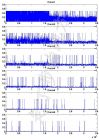
关于瞬时频率估计,前面虽说暂时放一下,但心中始终还是念念不忘,因为这是一道绕不过去的坎。在网上多次搜索、了解其现状。感觉是关注这件事的人很多,方法很多,但问题也很多。在网上能找到的方法,简单归结如下: 相位差分法 相位建模法 Teager能量算子法 跨零点法 求根估计法 反余弦法 时频分布法(谱峰检测法?) Shekel方法 Teager-Kaiser方法 解析信号法(HHT法) 其中有些只适用于单分量信号估计,有些可适用于多分量信号估计。由于单分量信号是多分量信号的特例,所以后者包括前者。 这些方法,有些我目前只能找到其名字,找不到原理论述;有些可以找到原理论述,但绝大多数方法都找不到现成的程序(收费网站内情况未知)。可以说,这些方法大多都只是用来写写文章、做做脑保健操而已,实际使用的人很少。如网上找到的一则“反余弦法瞬时频率估计”程序(见“附一”),它把分析信号的幅值都“规一化”了,因此它只能处理理想中的“平稳信号”,不能处理现实中的“非平稳信号”。 比较起来,现在使用解析信号法(HHT)估计瞬时频率的人是最多的,大有“众望所归”的趋势。此方法就是本人在前几篇博文中使用的方法。可是,它存在的问题,我在博文《18、关于IMF分量瞬时频率跳变问题的研究》也说的很详细了。既然现在最流行、影响最大的瞬时频率估计法都是这样,因此我有理由对其它所有瞬时频率估计方法,都感到没有信心。 解析信号法(HHT)估计瞬时频率用的是hhspectrum函数,hhspectrum函数是通过调用时频工具箱中的instfreq函数来进行瞬时频率估计的。时频工具箱中还有一个使用AR(2)模型进行瞬时频率估计的函数ifestar2(因为除却注释部分,程序正文很短,所以我把它也附在后面,方便阅读。见“附二”)。 现在来看看用ifestar2函数估计脉搏序列各IMF的瞬时频率: imfMBrd=emd(MB2917_rd); imfMBrd=imfMBrd'; lx=size(imfMBrd,1); for i=1:size(imfMBrd,2)-1; x=imfMBrd(:,i); =ifestar2(x); M{i,1}=fnorm; M{i,2}=t; M{i,3}=rejratio; end fid1=figure(1); set(fid1,'position', ) li=6; lj=1; for i=1:li for j=1:lj n=(i-1)*lj+j; s(n)=subplot(li,lj,n); set(s(n),'position', ); plot(M{n,2},M{n,1}) xlim( ) title( ) end end 运行 得 图30-1 fid2=figure(2); set(fid2,'position', ) li=7;% lj=1; for i=1:li for j=1:lj n=(i-1)*lj+j; s(n)=subplot(li,lj,n); set(s(n),'position', ); plot(M{n+6,2},M{n+6,1}) xlim( ) title( ) end end 运行得 图30-2 可见,IMF除了第10、第13分量以外,瞬时频率都有很严重的“跳变”,比HHT法更严重。从接近“0Hz”频率的地方跳到“0.5Hz”附近,如果都是这样还比较好区分,但那些比“0.25Hz”稍高的频率,你怎么知道它是否经过跳变呢?如果不是,那多大的频率是由负频跳变而来?界限在哪里?从物理意义来讲,正频率与负频率是截然不同的频率,一个是正向旋转所形成,一个是负向旋转所形成。频率表示方法,这是人类创造的理论,不管现实如何,用“0.49Hz”来表示“-0.01Hz”,这就叫“削足适履”。 以前多次讲过,现实信号的频率,一般情况下应该是连续、光滑的,所以我们的频率表示方法好不好,也应该以此为最高准则,是正频率就表示为正频率,是负频率就表示为负频率。除非能证明现实信号频率的确发生了跳变,否则频率表示当中出现了“跳变”,都是不对的。 下面将前面两张图的时间轴放大看看: fid3=figure(3); set(fid3,'position', ) li=6; lj=1; for i=1:li for j=1:lj n=(i-1)*lj+j; s(n)=subplot(li,lj,n); set(s(n),'position', ); stem(M{n,2},M{n,1}) xlim( ) title( ) end end 运行 得 图30-3 fid4=figure(4); set(fid4,'position', ) li=7; lj=1; for i=1:li for j=1:lj n=(i-1)*lj+j; s(n)=subplot(li,lj,n); set(s(n),'position', ); stem(M{n+6,2},M{n+6,1}) xlim( ) title( ) end end 图30-4 可以看到,图30-3的第1、第2分量频率、图30-4的第1分量频率,都有采样点上没有频率值的情况发生(不是“0Hz”情况哦)。其实每一个分量中都有这样的“瞬时频率无定义点”,只是因为在同一个绘图窗口将它们都绘出来不方便,所以就免了。 for i=1:size(imfMBrd,2)-1; lf(i)=length(M{i,1}) lt(i)=length(M{i,2}) rj(i)=M{i,3} end lf lt rj lf = Columns 1 through 7 33143345893484334901349453496134980 Columns 8 through 13 349933499335001350003499935001 lt = Columns 1 through 7 33143345893484334901349453496134980 Columns 8 through 13 349933499335001350003499935001 rj = Columns 1 through 8 0.94690.9882 0.9955 0.9971 0.9984 0.9989 0.9994 0.9998 Columns 9 through 13 0.99981.0000 1.0000 0.9999 1.0000 lf、lt是各IMF分量作了频率估算的频率点、采样点长度,rj是作了频率估算的采样点长度占整个采样点长度的比例。 这是由ifestar2函数中的indices = find(den0)造成的。与“反余弦法瞬时频率估计”一样,它能作频率估算的地方,它就作了估算;它无法作估算的地方,它就搁那不管了。这是什么态度嘛! 附一:网上找到的“反余弦法瞬时频率估计”程序代码 function = faacos(data, dt) % The function FAACOS generates an arccosine frequency and amplitude % of previously normalized data(n,k), where n is the length of the % time series and k is the number of IMFs. % % FAACOS finds the frequency by applying % the arccosine function to the normalized data and % checking the points where slope of arccosine phase changes. % Nature of the procedure suggests not to use the function % to process the residue component. % % Calling sequence- % = faacos(data, dt) % % Input- % data - 2-D matrix of IMF components % dt - time increment per point % Output- % f - 2-D matrix f(n,k) that specifies frequency % a - 2-D matrix a(n,k) that specifies amplitude % % Used by- % FA % Kenneth Arnold (NASA GSFC) Summer 2003, Initial %----- Get dimensions = size(data); %----- Flip data if necessary flipped=0; if (npts nimf) flipped=1; data=data'; = size(data); end %----- Input is normalized, so assume that amplitude is always 1 a = ones(npts,nimf); %----- Mark points that are above 1 as invalid (Not a Number) data(find(abs(data)1)) = NaN; %----- Process each IMF for c=1:nimf %----- Compute "phase" by arccosine acphase = acos(data(:,c)); %----- Mark points where slope of arccosine phase changes as invalid for i=2:npts-1 prev = data(i-1,c); cur = data(i,c); next = data(i+1,c); if (prev cur cur next) | (prev cur cur next) acphase(i) = NaN; end end %----- Get phase differential frequency acfreq = abs(diff(acphase))/(2*pi*dt); %----- Mark points with negative frequency as invalid acfreq(find(acfreq0)) = NaN; %----- Fill in invalid points using a spline legit = find(~isnan(acfreq)); if (length(legit) npts) f(:,c) = spline(legit, acfreq(legit), 1:npts)'; else f(:,c) = acfreq; end end %----- Flip again if data was flipped at the beginning if (flipped) f=f'; a=a'; end end 附二 时频工具箱中瞬时频率估计函数ifestar2 function =ifestar2(x,t); %IFESTAR2 Instantaneous frequency estimation using AR2 modelisation. % =IFESTAR2(X,T) computes an estimate of the % instantaneous frequency of the real signal X at time %instant(s) T. The result FNORM lies between 0.0 and 0.5. This %estimate is based only on the 4 last signal points, and has %therefore an approximate delay of 2.5 points. % %X : real signal to be analyzed. %T : Time instants (must be greater than 4) %(default : 4:length(X)). %FNORM : Output (normalized) instantaneous frequency. %T2 : Time instants coresponding to FNORM. Since the %algorithm can not always give a value, T2 is %different of T. % RATIO : proportion of instants where the algorithm yields %an estimation % %Examples : % =fmlin(50,0.05,0.3,5); x=real(x); =ifestar2(x); % plot(t,if(t),t,if2); % % N=1100; =fmconst(N,0.05); deter=real(deter); % noise=randn(N,1); NbSNR=101; SNR=linspace(0,100,NbSNR); % for iSNR=1:NbSNR, % sig=sigmerge(deter,noise,SNR(iSNR)); % =ifestar2(sig); % EQM(iSNR)=norm(if(t)-if2)^2 / length(t) ; % end; % subplot(211); plot(SNR,-10.0 * log10(EQM)); grid; % xlabel('SNR'); ylabel('-10 log10(EQM)'); % subplot(212); plot(SNR,ratio); grid; % xlabel('SNR'); ylabel('ratio'); % % See also INSTFREQ, KAYTTH, SGRPDLAY. %F. Auger, April 1996. % This estimator is the causal version of the estimator called % "4 points Prony estimator" in the article "Instantaneous %frequency estimation using linear prediction with comparisons %to the dESAs", IEEE Signal Processing Letters, Vo 3, No 2, p %54-56, February 1996. %Copyright (c) 1996 by CNRS (France). % % This program is free software; you can redistribute it and/or modify % it under the terms of the GNU General Public License as published by % the Free Software Foundation; either version 2 of the License, or % (at your option) any later version. % % This program is distributed in the hope that it will be useful, % but WITHOUT ANY WARRANTY; without even the implied warranty of % MERCHANTABILITY or FITNESS FOR A PARTICULAR PURPOSE. See the % GNU General Public License for more details. % % You should have received a copy of the GNU General Public License % along with this program; if not, write to the Free Software % Foundation, Inc., 51 Franklin St, Fifth Floor, Boston, MA 02110-1301 USA if (nargin == 0), error('At least one parameter required'); end; = size(x); if (xcol~=1), error('X must have only one column'); end x = real(x); if (nargin == 1), t=4:xrow; end; = size(t); if (trow~=1), error('T must have only one row'); elseif min(t)4, error('The smallest value of T must be greater than 4'); end; Kappa = x(t-1) .* x(t-2) - x(t ) .* x(t-3) ; psi1 = x(t-1) .* x(t-1) - x(t ) .* x(t-2) ; psi2 = x(t-2) .* x(t-2) - x(t-1) .* x(t-3) ; den = psi1 .* psi2 ; indices = find(den0); arg=0.5*Kappa(indices)./sqrt(den(indices)); indarg=find(abs(arg)1); arg(indarg)=sign(arg(indarg)); fnorm = acos(arg)/(2.0*pi); rejratio = length(indices)/length(t); t = t(indices); end (本文首发于: http://blog.sina.com.cn/s/blog_6ad0d3de01016a4n.html 首发时间:2012-06-07 20:40:45)
 标签: 瞬时频率估计