原文地址: http://blog.csdn.net/qiupingzhao/article/details/53171942 随机相位导致相干斑 一副影像的相位是随机的,原因: One pixel of a radar image usually represents a surface of several tens of square meters, containing numerous elementary targets (stones, branches, etc.). These targets all contribute to the signal and are located at different ranges from the radar. Since the wavelength is much smaller than the size of the pixel, the phase of a given target may be shifted by any value. The combination of these targets further randomizes the phase of the pixel. Clearly, no one value is statistically more significant than another. As far as amplitude is concerned, the contributions of two identical targets found in the same pixel can reinforce each other if their phases are identical or cancel each other out if they are opposite. The summing of the random phase values of these various targets produces the phenomenon known as ‘speckle’. If the same targets were arranged differently in another pixel they might produce a significantly different amplitude and an unpredictably different phase. 所以这样的相位信息没有办法加以利用,不过,两个这样的影像或许可以: If we want to use the phase of the signal as a measuring technique, the trick is above all to fully comprehend what is meant by ‘random’. A pixel phase is random because we do not know where the elementary targets are located within it. But on a second pass over the same pixel in exactly the same conditions we would of course obtain the same phase. Interferometry depends on the idea that, instead of using the phase of a radar image to measure the ranges, we can use the difference of phase between two radar images to measure differences or geometric distortions in range between these two images. We therefore count on the fact that the complex contribution depending on the particular arrangement of elementary targets in each pixel will be cancelled by combining the two images. 突然之间,我们会喜欢上这种随机,但是,我们希望这种随机在两幅影像上一致,只有这样才能够相互抵消,要不然仍然是可怕的随机。(就像上帝掷骰子一样,随机性有时候会让人觉得恐怖。) 这种能够”be cancelled”的能力,另一种说法就是相干。 事实上两幅影像是不可能 “in exactly the same conditions” 的: The two images which are merged point by point to form the image of their phase differences, called an interferogram, usually have different viewpoints because they were not taken from exactly the same place, and a time shift because they were not taken at the same moment. These two differences are almost always found in an interferogram. There may be no time difference in the case of systems with two radar antennas which can create two images simultaneously. In certain circumstances there may be no difference in viewpoint, if a satellite repasses at almost exactly the same point when acquiring the second image. These two differences are the source of the two types of information provided by interferometry. The difference of viewpoint provides the topographical information in the interferogram. The time difference provides information on displacement. 最后说说相干斑speckle: Homogeneous areas of terrain that extend across many SAR resolution cells (imagine, for example, a large agricultural field covered by one type of cultivation) are imaged with different amplitudes in different resolution cells. The visual effect is a sort of ‘salt and pepper’ screen superimposed on a uniform amplitude image. This speckle effect is a direct consequence of the superposition of the signals reflected by many small elementary scatterers (those with a dimension comparable to the radar wavelength) within the resolution cell. These signals, which have random phase because of multiple reflections between scatterers, add to the directly reflected radiation. From an intuitive point of view, the resulting amplitude will depend on the imbalance between signals with positive and negative sign. 对付相干斑的办法: Typically, image segmentation suffers severely from speckle. However, by taking more images of the same area at different times or from slightly different look angles, speckle can be greatly reduced: averaging several images tends to cancel out the random amplitude variability and leave the uniform amplitude level unchanged. 但这个方法能否用在干涉之前呢?似乎不能,是不是可能破坏掉相位信息? 相干与critical baseline 上面提到:这种能够”be cancelled”的能力,另一种说法就是相干。 实际上,衡量这种能力的指标叫相干系数。 An InSAR coherence image is a cross-correlation product derived from two co-registered complex-valued (both intensity and phase components) SAR images. It depicts changes in backscattering characteristics on the scale of the radar wavelength. Loss of InSAR coherence is often referred to as decorrelation. 相干性跟许多因素有关,其中一种是,基线,(垂直)基线越长,相干性会下降,当相干性完全消失时对应的垂直基线是critical baseline。这个定义还有很多其他的推导方式。它与波长、斜距、带宽、倾角、坡度角和光速有关。 关于critical baseline,另外一种解释方式,一个像素内部的各个目标的相位变化不应该因为基线(过大)而发生超过一个周期的差异: Let us take two distinct targets A and B, located at opposite edges of the same pixel in a reference image (one near the radar, the second further away). Targets A and B are indistinguishable within the pixel. Any elementary target in the pixel is subject to phase variations when passing from one image to another. The phase difference of the same pixel in M and S should not depend too much on the position of the target within the pixel. For instance, the phase difference itself should vary by much less than a full cycle between A and B. The overall phase difference resulting from the mixing of points P at various locations in the pixel will be insignificant at the scale of the pixel as long as the difference in δ (called the horizontal baseline) remains less than a limiting value. If this is not the case, the phase difference between the two images will again be the result of contributions which are random since they can vary within the pixel itself by more than a cycle. It will then be impossible to exploit this phase difference. For the limiting case where the targets are located at opposite edges of the pixel, the stability of the phase difference will be guaranteed by the stability of the incidence angle of the wave between the two images. Should this change too much, the path difference between the two targets in one image will differ from the path difference in the other image by more than a wavelength, resulting in a pure random difference of phase. For example, a 10-m ground pixel observed from an incidence angle of 30 implies a round trip path difference of 10 m between two targets at opposite edges of the pixel. If we wish to limit the variation of this path difference to a fraction of the wavelength, for example 1 cm, then the incidence angle in the second image must be between 29.967 and 30.033 A clearer way of quantifying this condition is to express the maximum acceptable horizontal distance δ between the points from which the images are acquired (also called the horizontal critical baseline, and deduced from the critical orthogonal baseline). For a satellite like ERS orbiting at an altitude of approximately 1000 km, this distance δ is about 1 km. In practice, we can only combine images separated by an integer number of satellite orbital cycles. The satellite is supposed to return to exactly the same position after each cycle. In most cases, it is actually less than 1 km away. Critical baseline 的第三种解释方式是主辅影像间的距离向频谱偏移 相位噪声 与相干性有关的另一个概念是相位噪声phase noise,这跟上面的问题其实联系得非常紧密,毕竟一幅影像也是复数,也是包括大小和相位的。 In the previous sections it has been hypothesised that only one dominant stable scatterer was present in each resolution cell. This is seldom the case in reality. We should analyse the situation where many elementary scatterers are present in each resolution cell (distributed scatterers), each of which may change in the time interval between two SAR acquisitions. The main effect of the presence of many scatterers per resolution cell and their changes in time is the introduction of phase noise. Three main contributions to the phase noise should be taken into consideration: 关于第二个,没错,基线会带来相位噪声,但是正是因为基线的存在,才能够进行地形测量。这里的spectral shift 方法在处理相位噪声的时候,会不会影响到有用的干涉相位? P45(靳)中分析得到的频谱相差正是能够进行地形测量的原因吧?应该不能完全去除? 答,这里的相位噪声来自于:the different combination of elementary (一个像素之内的),所以这里是不是只是在尽力去除掉一个像素内部的频谱偏移呢?(P18 practical approach) 还是说频谱偏移本身就是个坏东西,应该完全避免,我们的干涉测量并不会利用到频谱偏移?(仔细想想干涉测量的原理,根本原理是距离差对应相位差,跟频率似乎没有什么关系。另一方面,频率的变化势必会造成相位的变化,也就是说记录数据的相位不准确。) **以上的解释见“Range spectral shift”部分: 这个频谱偏移会导致失相关 是个坏东西 应该消灭掉 他代表的是相位随着斜距的变化 是由于视角差造成的 如果没有视角差 就没有干涉相位(或者说干涉相位是零,这里不考虑形变) 自然也就没有干涉相位的变化 这个视角差使得我们能够通过干涉相位进行地形测绘,但她同时导致了干涉相位的变化这个“副产品”。我们应该消除掉这个副产品,他和干涉相位不是一回事儿。** The phase noise can be estimated from the interferometric SAR pair by means of the local coherence γ. The local coherence is the cross-correlation coefficient of the SAR image pair estimated over a small window (a few pixels in range and azimuth), once all the deterministic phase components (mainly due to the terrain elevation) are compensated for. The deterministic phase components in such a small window are, as a first approximation, linear both in azimuth and slant-range. Thus, they can be estimated from the interferogram itself by means of well-known methods of frequency detection of complex sinusoids in noise (e.g. 2-D Fast Fourier Transform (FFT)). The coherence map of the scene is then formed by computing the absolute value of γ on a moving window that covers the whole SAR image. 相位噪声(The phase dispersion)可以表达为相干系数γ的函数,The phase dispersion can be exploited to estimate the theoretical elevation dispersion (limited to the high spatial frequencies) of a DEM generated from SAR interferometry. 相位噪声、相干、滤波、以及 covariance matrix estimation 之间的关系 将在后续详细分析。
原文地址: http://blog.csdn.net/qiupingzhao/article/details/53154348 Range spectral shift这个问题在斜坡效应中其实已经说过了。理解这个问题的关键在于: 知道频率是相位的微分(但这个(干涉数据的)频率跟载频、采样频率等其他的频率并不能混为一谈)。这样就能够很好地理解“斜坡效应”部分根据频谱偏移的公式解释条纹密度随着地形坡度的关系,因为频谱偏移本质上就对应相位变化; 观测视角的变化对应频率的变化; 这个问题和斜坡效应、失相关以及critical baseline都是相通的 频谱偏移和相位梯度那些事儿(由此导出了一个条件限制) Other sources of decorrelation are more significant and non-reversible. The two most important conditions are related to the phase gradient and the temporal variation in the physical distribution of the elementary scatterers. The phase gradient condition can be conveniently described in the spectral domain. The temporal bandwidth of the SAR images in range corresponds with a spatial bandwidth due to the projection on the earth’s surface. A phase gradient in range of n cycles/pixel corresponds with a spectral shift between the spectra of both acquisitions of n*f Hz, where f is the sampling frequency. The spectral shift results in a decreased overlap between the corresponding parts of the spectrum (the signal) and an increasing non-overlapping part of the spectrum (the noise). Due to the limited bandwidth, a phase gradient larger than B/f cycles/pixel (approximately 0.822 for ERS) results in a zero overlap between the spectra, hence a complete loss of correlation. The occurrence of this situation is dependent on: the length of the perpendicular baseline, the steepness of the topographic slopes, and/or the gradient of the surface deformation. 说明 理一理这里的逻辑: 这个频谱偏移会导致失相关 是个坏东西 应该消灭掉 他代表的是相位随着斜距的变化 是由于视角差造成的 如果没有视角差 就没有干涉相位(或者说干涉相位是零,这里不考虑形变) 自然也就没有干涉相位的变化 这个视角差使得我们能够通过干涉相位进行地形测绘,但她同时导致了干涉相位的变化这个“副产品”。我们应该消除掉这个副产品,他和干涉相位不是一回事儿。 以上说明了Range spectral shift的由来 那么怎么进行滤波呢? 参考文献 Hooper, A., Bekaert, D., Spaans, K., Arıkan, M. (2012). Recent advances in SAR interferometry time series analysis for measuring crustal deformation. Tectonophysics, 514, 1-13. Zhong, L., Dzurisin, D. (2014). Insar imaging of aleutian volcanoes. Springer Praxis Books, 2014(8), 1778–1786. Ketelaar, V. (2009). Satellite radar interferometry : subsidence monitoring techniques.
在信号与系统中,我们经常会遇到对于一个信号 s ( t ) = cos ( ω t + θ ) , 乘上一个复数 e j ϕ ,即 s ( t ) ∗ e j ϕ 表示对原信号 s ( t ) 移动相位 ϕ 。 那么如何理解乘上一个 e j ϕ 可以表示相位的移动呢? 这里需要用到欧拉公式,具体可以参看我另外一篇博文: 欧拉公式 cos ( ω t + ( θ + ϕ ) ) = R e { e j ( ω t + ( θ + ϕ ) ) } = R e { e j ( ω t + θ ) e j ϕ } 可以看到,在原信号上叠加一个相位 ϕ 相当于在原信号上乘以一个复数 e j ϕ ,注意这里信号是取的实部。 更进一步,我们在几何上解释一下复数与相位(旋转)的关系。 如下图所示,横坐标为实部,纵坐标为虚部,有两个单位向量 a , b ,其中 a = e j θ ,那么向量 b 该如何表示呢? 由欧拉公式 e j θ = cos ( θ ) + j sin ( θ ) ,则 a 可以表示为 ( cos ( θ ) , sin ( θ ) ) ,这个我们从图中也可以很轻松的得到。由图中的角度关系,我们可以得到 b = ( cos ( θ + ϕ ) , sin ( θ + ϕ ) ) ,写成复数形式,即 b = e j θ e j ϕ = e j ( θ + ϕ ) 。可以很明显的看到,对向量 a 乘上一个 e j ϕ 表示将 a 旋转角度 ϕ ,即相位移动 ϕ 。
1985年发表的论文,信息如下: G. R. Olhoeft (1985).”Low-frequency electrical properties.” Geophysics, 50(12), 2492-2503. doi: 10.1190/1.1441880 In the interpretation of induced polarization data, it is commonly assumed that metallic mineral polarization dominantly or solely causes the observed response. However, at low frequencies, there is a variety of active chemical processes which involve the movement or transfer of electrical charge. Measurements of electrical properties at low frequencies (such as induced polarization) observe such movement of charge and thus monitor many geochemical processes at a distance. Examples in which this has been done include oxidation‐reduction of metallic minerals such as sulfides, cation exchange on clays, and a variety of clay‐organic reactions relevant to problems in toxic waste disposal and petroleum exploration. By using both the frequency dependence and nonlinear character of the complex resistivity spectrum, these reactions may be distinguished from each other and from barren or reactionless materials Read More: http://library.seg.org/doi/abs/10.1190/1.1441880 前5年只获得8次引用,平均每年获得1.6次引用。 James A. Tyburczy , Jeffery J. Roberts . (1990) Low frequency electrical response of polycrystalline olivine compacts: Grain boundary transport. Geophysical Research Letters 17 , 1985-1988. Online publication date: 1-Oct-1990. CrossRef Andrew K. Jonscher . (1990) Admittance spectroscopy of systems showing low-frequency dispersion. Electrochimica Acta 35 , 1595-1600. Online publication date: 1-Oct-1990. CrossRef J.R. Wait . 1989. COMPLEX RESISTIVITY OF THE EARTH. Progress in Electromagnetics Research, 1-173. CrossRef R. S. SMITH , P. W. WALKER , B. D. POLZER , G. F. WEST . (1988) THE TIME-DOMAIN ELECTROMAGNETIC RESPONSE OF POLARIZABLE BODIES: AN APPROXIMATE CONVOLUTION ALGORITHM1. Geophysical Prospecting 36 :10.1111/gpr.1988.36.issue-7, 772-785. Online publication date: 1-Oct-1988. CrossRef Richard S. Smith , G. F. West . (1988) An explanation of abnormal TEM responses: coincident-loop negatives, and the loop effect.. Exploration Geophysics 19 :3, 435-446. Online publication date: 1-Sep-1988. Abstract | PDF (1210 KB) | PDF w/Links (747 KB) A. Duba , E. Huengest , G. Nover , G. Will , H. Jodicke . (1988) Impedance of black shale from Munsterland 1 borehole: an anomalously good conductor?. Geophysical Journal International 94 , 413-419. Online publication date: 1-Sep-1988. CrossRef Alan D. Chave , John R. Booker . (1987) Electromagnetic induction studies. Reviews of Geophysics 25 , 989. Online publication date: 1-Jan-1987. CrossRef David A. Lockner , James D. Byerlee . (1986) Changes in complex resistivity during creep in granite. Pure and Applied Geophysics PAGEOPH 124 , 659-676. Online publication date: 1-Jan-1986. CrossRef Read More: http://library.seg.org/doi/abs/10.1190/1.1441880 2014年获得9次引用 2013年获得14次引用,大大超过了论文发表后5年内引用数的总和。 2012年获得7次引用 2011年获得16次引用 2010年获得9次引用 最近5年获得55次引用,大约等于论文发表后5年内引用数的7倍。 引用数激增的原因在于近年来出现了高精度岩石物理性质测量仪器,用新仪器可以发现以前无法观测到的现象,岩石物理又火起来了。
 标签: 相位