原载 http://blog.sina.com.cn/s/blog_729a92140102vz7w.html 由于某些原因,人们在应用实践中,常未明确考虑基于连续时间小波基函数的被处理数据初始化问题,或无交代,甚至有人误以为Mallat算法就已解决了这一问题。有研究者,对此状况,持较严厉的批评态度,于是有“小波罪恶(wavelet crime)”之说,如图片1的顶部所示。 把离散变换和连续时间信号联系起来,可以更好地理解和开拓应用,但这样常不得不接受近似处理。在与Mallat算法有关的小波变换中,过渡联系的麻烦,表现得尤其突出,难被消除。严格地说,在很多实践中,紧支集连续时间小波基函数,还不算真有用。 习惯于傅立叶分析时,可能想,用矩形窗截取FIR低通滤波器序列的傅立叶变换的一个周期,然后利用频谱的伸缩以获得不同的低通带宽度,就得意味着不同分辨率的子空间簇。然而实际上,在Mallat等的连续时间能量有限信号空间的多分辨分析理论中,尺度函数以及嵌套子空间列,有非直观的特殊的定义方式。人们常难由FIR滤波器组用闭式表达连续时间基函数,只知在极限意义上存在,一个具有某些性质的连续时间尺度函数和小波函数系。 即使,可用解析式表示被处理信号,也不一定容易计算出它与某个紧支集基本函数的平移系的内积,更何况,实际应用中常常只知离散序列 (名著“十讲”第五章后的注释 12,是研究初始化滤波的引子), 难确定其对应的合适函数子空间。这个内积,是连续时间基函数的应用解释的严密性的关键,而也反使数字频率与模拟信号物理频率的精确联系变得麻烦。 如果什么都已知的话,也许 人们 就不需离散小波变换,来做压缩或降噪等事情了。 见到Matlab小波工具箱通过数字计算画个小波函数曲线时,也不清楚其中局部扭结小尖峰,正是好的性质的体现,还是有了较多数字误差。 居士脱离连续时间,直接讨论离散小波包变换,可以使计算理论更独立严谨。这正如,离散傅立叶变换及其快速算法,不必依赖于,连续时间和连续频率概念。由离散时间滤波器组,进入某些函数空间,在其中做理论分析等,是其它的故事。不同的部分,各有价值。 某些问题还未解决好,或未被意识到,或者论述行文失误,都是研发中较常见的事,不意味着“犯罪或邪恶”。这正如,不能说,应用傅立叶变换或Shannon采样定理时的不都定量的近似,是“违法”行为。现代的傅立叶变换理论,已包括很多部分,在数字计算中实际常用的是FFT。各部分连接的关键基础,在长时间的大量文献中 , 同样可能有“不尽人意”之处。当然,批评与自我批评,有事说事,努力解决问题,这是正道。 在傅立叶让他的级数出世后,人们用了相当长的时间,理清傅立叶级数的收敛性问题。 图片1.中关于采样定理的描述,取于国内外的著名教科书或著作,并不是研发初学者之作。 看起来,不算“明确而精辟”。 为什么不用开区间,表示信号的频谱?直观地看:采样使频谱周期延拓时,闭区间有重叠点,使“离散谱”混叠、消失、或不能区分两个边界频率;而且,理想滤波器的频响,在边界频率处不连续,使人感到,不确定、不安全、宜避开。开区间,至少从形式上就排除了麻烦:在边界频率上的正弦信号一个周期内,正好都采到零。 为什么不用半开半闭区间,表示信号的频谱?直观地看:频谱周期延拓时,可无重叠点,也包括了整个频率轴,更像是在频谱的采样离散化时单个周期的两端点中只取一侧。 早期的采样定理中的信号及其傅立叶变换,到底需要什么严格条件? 维基百科,并不排除,定理适用于频率在边界以内的正弦信号(如文后附1.)。“教育部研究生工作办公室推荐研究生教学用书”《数字信号处理》,有专节讨论正弦信号抽样的问题。更一般地讲,定理要面对离散频率成分的问题。 绝对可积函数的傅立叶积分变换,或连续频谱函数,不适用于正弦波。像Dr.Daubechies那样,把带限信号集,视为能量有限 (无穷时间) 信号空间的子空间,陈述采样定理时,也排除了正弦函数等功率有限而能量无限的周期信号。 使用冲激函数串来推演采样定理,这意味着引入了广义函数的傅立叶变换。统一表达了离散谱线和连续区间上的频谱之后,定理就包括了正弦函数。 现在相信,实际信号都是能量有限的,不存在无始无终的永动机式的精确单频率运动过程,人们天天做的采样、数-模转换、滤波都是现实的。然而,信号分析实验中常用的三角函数模型和采样定理中的sinc插值重建函数,都不是物理可实现的。 即使,认为现实中能记录的信号,都既是时限的也是带限的,也不都很精确每个实际问题中的误差,一般也不随Slepian等研究“时-频限”。很多时候,也未必明确所谓的冲激函数串的理想化抽象近似的量度。 Shannon采样理论,用sinc函数做 理想 插值重建(Whittaker–Shannon interpolation formula),违背因果律。很强调了带限,削弱了对现实时限的注意。实际上,采样率变化了,那么,某给定时间区间内的重建信号,受该区间外的样本点影响的程度,也就不同了。假如对插值函数做截断近似,则还需要兼顾函数值的量化误差。 至此,容易注意到,过采样的采样率很高时,可以认为很多“插值函数、重建基函数”都可“更近似于冲激函数”,其差别减小了。这样,使用多分辨分析子空间的小波变换的初始化时,误差也可能减小。 记得当年老师说,凭经验,实用电路中,采样频率一般大于信号成分的最高频率的2.5倍,因为低通模拟滤波器的过渡带不是理想的。田边顽童,不识定理,更无非均匀采样理论,而可能用小石子或谷粒拼出些自以为像人头的图案,指指点点,叫这个狗娃,称那个胖仔。 新浪赛特居士SciteJushi-2015-11-22。 图片 1.小波罪恶之说与采样定理的表述 附 1:Wikipedia中的采样定理(Nyquist–Shannon sampling theorem) 部分的摘录 Sampling is the process of converting a signal (for example, a function of continuous time and/or space) into a numeric sequence (a function of discrete time and/or space). Shannon's version of the theorem states: If a function x(t) contains no frequencies higher than B hertz, it is completely determined by giving its ordinates at a series of points spaced 1/(2 B ) seconds apart. A sufficient sample-rate is therefore 2 B samples/second, or anything larger. Equivalently, for a given sample rate f s , perfect reconstruction is guaranteed possible for a bandlimit B ≤ f s /2. When the bandlimit is too high (or there is no bandlimit), the reconstruction exhibits imperfections known as aliasing. Modern statements of the theorem are sometimes careful to explicitly state that x ( t ) must contain no sinusoidal component at exactly frequency B , or that B must be strictly less than ½ the sample rate. The two thresholds, 2 B and f s /2 are respectively called the Nyquist rate and Nyquist frequency . And respectively, they are attributes of x ( t ) and of the sampling equipment. The condition described by these inequalities is called the Nyquist criterion , or sometimes the Raabe condition . The theorem is also applicable to functions of other domains, such as space, in the case of a digitized image. The only change, in the case of other domains, is the units of measure applied to t , f s , and B .
芝诺“飞矢不动”的悖论说:飞行的箭,每个时刻都占据了一个确定的位置,这意味着它不会同时存在其他的位置,箭矢的位置固定,所以它在这时刻是静止的。依此推理,飞行的箭在任何时刻都是静止的,所以运动在逻辑上是不可能的。 对于这个悖论,有不同的解答。黑格尔认为运动就是一对矛盾,每个时刻飞矢是既在这个位置又不在这个位置上,用辩证法回避了形而上学的挖掘。康德认为时间和空间并非事物的属性,而是我们感知事物方式的属性,这个矛盾是我们过去时空观念的疵瑕。休谟否认时空的无限可分性,以此也可以给出有穷时空的离散化解释。而牛顿坚持了时空无穷可分的观点,用微积分给予近代的解释。从而也让时空无穷可分的假设变成了公认的真理。 运动在直观上是个时间段上位移的现象,当一个物体在时刻 t 0 到 t 1 的时段,从位置 x 0 到了 x 1 ,如果Δ t = t 1 -t 0 ≠ 0 时Δ x = x 1 -x 0 ≠ 0 ,我们说它是在运动。物体在这时段的速度为Δ x / Δ t ,意思是位移对时段里时间流逝的变化率。物体时刻 t 1 在位置 x 1 ,这个信息,不足以判定它是静止还是运动的。只要Δ t 0 ,速度Δ x/ Δ t ≠ 0 ,在 ,那么 D 的特征向量集合 $\{e_k=\frac{1}{\sqrt{2\pi}}e^{-ikt} \; | \; k \in \mathbb{Z} \}$ 便是这空间上的一个正交归一基。 让我们首先来验证正交归一性。对于 L 2 空间,它的内积定义是 $ \left \langle f{(\cdot)},g(\cdot) \right \rangle = \int_0^{2\pi}f(t)\overline{g(t)}dt$ ,对于任意整数 m,n ,我们有: $\left \langle \frac{1}{\sqrt{2\pi}}e^{-imt},\frac{1}{\sqrt{2\pi}}e^{-int}\right \rangle =\frac{1}{2\pi}\int_0^{2\pi}e^{-imt}e^{int}dt =\frac{1}{2\pi}\int_0^{2\pi}e^{-i(m-n)t}dt = \delta_{mn}$ 这就证明了它们是正交归一的。空间中向量 $f(\cdot)\in L^2 $ 在 e k 上的投影是: $\left \langle f(\cdot),e_k \right \rangle = \frac{1}{\sqrt{2\pi}}\int_0^{2\pi}f(t)e^{ikt}dt$ 这是大家熟悉的函数 $f(\cdot)$ 傅立叶系数的复数形式(若将复数展开成余弦和正弦正交基,则系数乘一个常数因子)。函数 $f(\cdot)$ 对这组向量的分解是傅立叶级数,不难证明这个傅立叶级数收敛于 $f(\cdot)$ 。所以它们构成了 L 2 空间上的基。经典的傅立叶级数,就是建立在微分算子 D 一组在 L 2 空间正交归一的特征向量上。这组可数的基张成了 L 2 希尔伯特空间。 注意到微分算子 D ,有不可数的特征向量 $e^{-iat}$ ,所以它们在无穷序列表达下可能是线性相关的。这取决于它们所在的空间。 是不是所有希尔伯特空间中的点都能表达成无穷级数?也就是说,是不是它们都有可数的基?答案是否定的。 例如:对于函数定义内积为$\left \langle f(\cdot),g(\cdot) \right \rangle = \lim_{T\rightarrow \infty}\frac{1}{T}\int_{-T\pi}^{T\pi} f(t)\overline{g(t)}dt$,它构造了一个希尔伯特空间$L^2(-\infty, \infty)*$,对所有的实数s,t的函数$e_s(t) = \frac{1}{\sqrt{2\pi}}e^{-ist} $都是这空间上线性算子D的特征向量,不难验证它们是正交归一的,这组向量是不可数的。 $L^2 $ 是可分的希尔伯特空间,里面的函数可以用傅立叶级数来表达(在 L 2 积分意义下收敛,级数展开几乎处处逐点收敛于它)。而 $L^2(-\infty, \infty)*$ 这希尔伯特空间是不可分的,所以这里的函数不能用傅立叶级数来表达。例子里那组向量是个不可数的正交归一基,这空间里的函数可以用积分变换来表达对这组基的分解和线性组合。从内积公式得到傅立叶变换,即是对这组基分解的分布函数;对基向量分布性分解的线性组合可直接写出傅立叶变换的反演。这提供了一个通俗的直观解读。更深入的探讨,诸如无穷区域的积分,无穷小分解系数分布函数的表达,积分的线性组合表示,及扩充到广义函数等等数学细节,在Sobolev空间可以得到更严谨的解读。 数学是直观想象在逻辑上精确化的学问。希尔伯特空间的研究,源自狄拉克对量子力学算符的表达。狄拉克非常注重数学上形式的美,简洁的美,他以此扩充了许多直观概念的应用场合,取得十分漂亮的结果。但在无穷世界的想象,还是需要用精确的逻辑来校正。 1927 年冯·诺依曼、希尔伯待和诺戴姆的论文《量子力学基础》,纠正了狄拉克缺乏严谨的不足。 在早期的泛函分析研究,特别是在物理应用中,希尔伯特空间指的是可分的完备的内积空间,即这空间有可数的稠集。上面的例子说明并非都是如此的。 大家已经熟悉在 $\mathbb{R}^n$ 空间上的微分,怎么将它推广到往整体看不是那么“平整”的空间?先看看平面几何是怎么使用的。我们生活的大地实际上是地球球面上的一部分,把这个局部当作 2 维的欧几里德空间,或者说映射到 $\mathbb{R}^2$ 空间。每一个局部地方在映射下对应着一个平面地图,球面上每个地点对应着平面地图上一个坐标,我们可以用坐标进行这个球面局部的各种计算。用几张平面地图覆盖了全球,就可以计算地球的各处。 对高维和更一般情况,也可以类似地,把拓扑空间 X 的一个局部开集,一一映射到 $\mathbb{R}^n$ 空间上来计算。 X 空间上的一个点 x 对应着 $\mathbb{R}^n$ 空间上的一个点,称为 x 的坐标, x 的邻域对应着坐标的邻域以保持对应的收敛关系。所以这个映射必须是同胚的,也就是这个一一对应的映射双向都是连续的,就像 X 中的这个开集通过伸缩变形展平成 $\mathbb{R}^n$ 空间的开集一样。如果有一族这样的开集覆盖了 X ,都能做到这样的映射,那么 X 上的每个点都有了 n 维实数的局部坐标。这样的 X 空间便称为 流形 。覆盖开集的重叠部分,流形上的点在不同映射的局部坐标系上,可以进行坐标变换。因为这样的映射是定义在开集上,所以 x 点总有一个足够小的邻域是完全在一个映射的局部坐标系上, x 点与它坐标的收敛关系是一一对应的,如果交集之处的坐标变换是连续可导的,整个流形通过这些映射的坐标系,便可以有对应的微积分计算,这时称为 微分流形 。 当然并非任何的拓扑空间都能做到这一点。流形 X 的拓扑不能太粗,对于两个点必须有能够分开的邻域,即是 T2 或者称为 Hausdorff 空间;拓扑也不能太复杂,要有可数的拓扑基(其元素的并能够生成所有开集,即是第二可数的)。局部映射必须与相同维数的 $\mathbb{R}^n$ 空间同胚。下面是用数学语言描述的定义。 X 是第二可数,T2的拓扑空间,若在一个覆盖X的开集族中的每个开集,都有一个嵌入$\mathbb{R}^n$的同胚映射,X可以称为 n维拓扑流形 ,这个映射称为 坐标图 。在拓扑流形上,两个坐标图交集部分的点在不同的坐标图上映成不同的(坐标)点,如果这两个坐标变换函数有r阶连续导数,则称它们是C r 相容的坐标图。如果所有坐标图都是C r 相容的,则称这个流形为 C r 微分流形 。r为无穷大时称为 光滑微分流形 。 对于一般的距离空间,它是 T2 ,但只是第一可数的。如果它还是可分的,则它是第二可数的,这个拓扑中任何的开集都能由一组可数开球,用它们的并集来构成。可分的距离空间满足第二可数和 T2 的条件,只要每点的开邻域都有同维数的同胚坐标映射,就可以是流形。 两个维数分别为 m 和 n 的 C r 微分流形间的映射称为 C r 映射,它可以表示为对应点局部坐标上的 C r 函数。对这个函数的求导和积分,对应着这两个流形间的映射在这局部区域上的相应的运算。比如说, n 维光滑微分流形 X 到 $\mathbb{R}$ 的函数,在 X 中点 x 的邻域对应着 $\mathbb{R}^n$ 空间上一段光滑曲线。这条光滑曲线,对应着 x 点的切线(用方向导数表示)是一个 n 维向量,所有这些切向量形成的空间称为 X 在 x 处的切空间。虽然上述的切空间是由某一局部坐标系下定义的,可以证明不同的坐标系导出的切空间是相同的。直观上可以想象成二维 X 曲面在 x 这一点上的切平面。如果一个映射 F 将 C r 微分流形 X 上每一点都对应着它切空间上的一个向量, F 称为 C r 向量场,在局部坐标下表示如下,其参数都是 C r 函数。 $F = \sum _{i=1}^n a_i(x)\frac{\partial }{\partial x_i}$ 纤维丛 的定义了包含三个拓扑空间 B , M , Y 和一个投影映射 p :基空间 M 是全空间 B 的投影 p(B)=M ;基空间上每一个点 x 对应着这个投影在全空间 B 里的原像 p -1 (x) ,这原像与丛空间 Y 同胚,称为这点上的丛;基空间上每一点存在着一个邻域 U ,直积空间 UxY 与 U 的投影原像 p -1 (U) 同胚。在直观上可以想象二维曲面 M ,每一点 x 上都有一根 p -1 (x) 的纤维,这些纤维互不相交,全体构成三维空间 B 。 B 中的每一点都可以沿着纤维对应到 M 的同一个点上(称为投影),全空间上点的邻域在纤维上和投影到基空间上仍然是它们的邻域。不要把基空间 M 想象成一把刷子的底部, M 应该看成是全空间的一个横截面,密实的纤维集束穿过这个横截面向两边无限延伸。每根纤维都像直线 Y 的弯曲变形。纤维丛的数学模型也可以用来描述物理空间中的场。 微分流形和纤维丛,若以欧几里德三维空间中的曲面和纤维集束几何体来看,都不难想象其图像。不过它们是在抽象的点集拓扑空间上有严格的定义,从而能够在上面推广微积分的应用。这些都是现代微分几何课程的内容,这里的简略介绍,希望通过较精确的数学定义,让大家可以想象这些概念。 (待续) 【扩展阅读】 冯·诺依曼关于量子理论的数学基础,算子环,遍历理论的研究 http://www.kepu.net.cn/gb/basic/szsx/2/25/2_25_1008.htm 钱诚德,高等量子力学 http://course.zjnu.cn/huangshihua/book/%E9%92%B1%E8%AF%9A%E5%BE%B7_%E9%AB%98%E7%AD%89%E9%87%8F%E5%AD%90%E5%8A%9B%E5%AD%A6.pdf 关肇直等,张恭庆,冯德兴,线性泛函分析入门,上海科学技术出版社, 1979 维基百科,流形 http://zh.wikipedia.org/wiki/%E6%B5%81%E5%BD%A2 程代展,系统与控制中的近代数学基础,北京:清华大学出版社, 2007 http://product.dangdang.com/9350967.html
8.倒格子空间 两位布拉格同时被授予诺贝尔物理奖,自然地引起了人们的质疑:这个工作恐怕主要是由父亲做的吧?这种说法不知是否也曾经使小布拉格苦恼过?他可能并不在乎,因为他有独自发表的第一篇论文,强烈地、毫无疑问地证明了他对这个领域的贡献和能力 【 2】 。 早在 6岁的孩童时代,1896年,小布拉格因为骑自行车摔跤 而受伤。父亲带儿子用当时澳大利亚新装配的第一台 X 射线发生器,拍了一张儿子肘部受伤部位的 x 射线照片。也许从那时候开始, 小布拉格就牢牢地记住了这位能干的 x-射线‘女士’? 1912 年,劳厄发表有关 X 射线衍射的论文时, 小布拉格正在剑桥大学做研究。 劳厄的工作立刻引起了 小布拉格的兴趣,不到四个月之后,他就以《晶体对短波长电磁波的衍射》为题向剑桥哲学学会报告了他的研究成果。 文章中,小布拉格成功地解释了劳厄的实验事实,提出了晶体衍射的布拉格方程,巧妙而方便地借用镜面反射规律来描述晶体中各原子对电磁波的衍射效应。不过,他在文章标题中用的是‘短波长电磁波’,而不是‘ X-射线’一词,这是为什么呢?其原因与老布拉格当时对X-射线的看法有关。开始时,老布拉格认为X-射线不是波,而是一种微粒,他试图用微粒理论来解释劳厄的照片,但失败了。布拉格一家人夏天在海滨度假的时候,父子俩讨论过这个问题。小布拉格回到剑桥后发现,如果用某种‘短波长电磁波’的概念,能够完美地解释劳厄观察到的现象。但是,受父亲观点的影响,小布拉格尚未确定这个短波长的电磁波,到底是入射的X-射线本身,还是X-射线通过晶体时激发产生出来的另一种次级电磁波。后来,老布拉格用实验观察证实了衍射后的出射波也是X-射线,才接受了X-射线就是一种电磁波的理论,转而和儿子一起,潜心研究晶体结构分析的实验方法,并对多种晶体进行了测试,奠定了用X-射线衍射来确定晶体结构的理论基础。 图 7 ( a )是晶体衍射的示意图。 根据布拉格衍射条件: 2 d sin θ = n λ ,这儿, d 是晶格常数, θ 是衍射角。 如果我们将波长 λ 用波矢量 k= 2p/l 来代替的话, 经过简单的代数变换后,很容易将 衍射条件 写成: k sin θ = n ( p/ d ) ( 7.1 ) 仔细观察图 7 ( a ),我们发现,不难从几何上理解公式( 7.1 )。它描述了满足衍射加强条件的波矢 k 与晶体结构中原子间距 d 之间的关系。满足衍射加强条件的波矢 k 的方向,也就是能打在衍射屏幕上而出现亮点的电磁波方向。所以,换言之,公式( 7.1 )描述了衍射图像亮点的位置与 d 之间的某种关系。什么样的关系呢?公式的右边是变量 ( p/ d ) 的整数倍,这个变量与原子间距离 d 的倒数有关。 图 7 再进一步引伸下去,说得更清楚一些。图 7(a)所示的衍射实验,得到如(b)图所示的衍射图像,这个图像看起来是某种格点空间的映像。这个新格点空间不是晶格本身,但是又和原来的晶格有关系:新格点间的距离正比于原来晶格原子间距d的倒数。而且,新格子空间的量纲也倒过来了。原来的晶格是在真实空间中,点间的距离d是长度(米)的量纲,而新格点间的距离 ( p/ d ) 的量纲是‘米’的倒数( 1/ 米)。 既然数值和量纲都是倒数的关系,人们便把这个虚拟的空间叫做 ‘倒格子’空间,见图 7(c)。 从数学的观点看,倒格子是原来周期性晶格的傅立叶变换 【 3】 。说到傅立叶变换,大家比较熟悉的是从时间空间到频率空间的变换,时间的周期函数变换成频谱。比如,我们用光谱来研究光线中包含的各种颜色,用乐谱来表示音乐。对晶体来说,傅立叶变换将通常的坐标空间变换成了波矢空间。而原来坐标空间中的晶格,则变换成了波矢空间中的‘倒格子’。无论是正格子,还是倒格子,都属于我们在前一节中提到过的‘ 布拉菲点阵’。并且, 正格子和倒格子在对称性方面互相关联,产生许多有趣的特性,在此不再赘述,读者可参考有关文献 【 4】 。 现在,我们知道晶体的衍射图像对应于倒格子,就更加明白了布拉格父子工作的重要意义。因为固体中原子的晶格结构,是很难用显微镜直接观察到的。但是, X射线的衍射图像却已经可以得到。从X射线的衍射图像,我们可以计算出倒空间的几何结构,然后,再从倒空间,反过来又能计算出正晶格的相关常数,这样,晶体的结构不就一目了然了吗。因此,波矢空间及倒格子的概念,对研究固体物理的意义非常重大。 探测晶体结构,不仅使用 X-射线,也能用电子或中子衍射,从量子力学的观点,这些粒子(或电磁波)都具有波粒二象性,波矢反映了波动性,粒子性则可用动量表示。波矢与动量之间只相差一个常数因子,因此,波矢空间有时也称为动量空间。 固体的晶格结构清楚了,就方便于从理论上求解薛定谔方程,从而研究电子在固体中的运动规律。这样,下一节我们又将返回到固体中电子能带的问题。 参考资料: 【 1】Bravais, A. (1850). Mémoiresur les systèmes formés par les points distribués régulièrement sur un plan oudans l'espace. J. Ecole Polytech. 19: 1–128 (English: Memoir 1,Crystallographic Society of America, 1949.) 【 2】Bragg, W.L. (1913). TheDiffraction of Short Electromagnetic Waves by a Crystal. Proceedings ofthe CambridgePhilosophical Society 17: 43–57. Bragg's Nobel lecture ''The diffraction of X-rays by crystals'' is at http://diamond.kist.re.kr/knowledge/nobel-physics/1915/wl-bragg-lecture.pdf The Nobel Prize in Physics 1915. Nobel Foundation。 【 3】B. E. Warren (1969/1990) X-raydiffraction (Addison-Wesley, Reading MA/Dover, Mineola NY). 【4】 《固体物理学》,黄昆、韩汝琦著,高等教育出版社出版, 2005, 上一篇:能级和能带(2) 系列科普目录 下一篇: 布洛赫波和布里渊区 8-x-diff.jpg
据MIT新闻网站报道,MIT的科学家研究出比FFT更快的傅立叶变换算法。 The Fourier transform is one of the most fundamental concepts in the information sciences. It’s a method for representing an irregular signal — such as the voltage fluctuations in the wire that connects an MP3 player to a loudspeaker — as a combination of pure frequencies. It’s universal in signal processing, but it can also be used to compress image and audio files, solve differential equations and price stock options, among other things. The reason the Fourier transform is so prevalent is an algorithm called the fast Fourier transform (FFT), devised in the mid-1960s, which made it practical to calculate Fourier transforms on the fly. Ever since the FFT was proposed, however, people have wondered whether an even faster algorithm could be found. At the Association for Computing Machinery’s Symposium on Discrete Algorithms (SODA) this week, a group of MIT researchers will present a new algorithm that, in a large range of practically important cases, improves on the fast Fourier transform. Under some circumstances, the improvement can be dramatic — a tenfold increase in speed. The new algorithm could be particularly useful for image compression, enabling, say, smartphones to wirelessly transmit large video files without draining their batteries or consuming their monthly bandwidth allotments. Like the FFT, the new algorithm works on digital signals. A digital signal is just a series of numbers — discrete samples of an analog signal, such as the sound of a musical instrument. The FFT takes a digital signal containing a certain number of samples and expresses it as the weighted sum of an equivalent number of frequencies. “Weighted” means that some of those frequencies count more toward the total than others. Indeed, many of the frequencies may have such low weights that they can be safely disregarded. That’s why the Fourier transform is useful for compression. An eight-by-eight block of pixels can be thought of as a 64-sample signal, and thus as the sum of 64 different frequencies. But as the researchers point out in their new paper, empirical studies show that on average, 57 of those frequencies can be discarded with minimal loss of image quality. Heavyweight division Signals whose Fourier transforms include a relatively small number of heavily weighted frequencies are called “sparse.” The new algorithm determines the weights of a signal’s most heavily weighted frequencies; the sparser the signal, the greater the speedup the algorithm provides. Indeed, if the signal is sparse enough, the algorithm can simply sample it randomly rather than reading it in its entirety. “In nature, most of the normal signals are sparse,” says Dina Katabi, one of the developers of the new algorithm. Consider, for instance, a recording of a piece of chamber music: The composite signal consists of only a few instruments each playing only one note at a time. A recording, on the other hand, of all possible instruments each playing all possible notes at once wouldn’t be sparse — but neither would it be a signal that anyone cares about. The new algorithm — which associate professor Katabi and professor Piotr Indyk, both of MIT’s Computer Science and Artificial Intelligence Laboratory (CSAIL), developed together with their students Eric Price and Haitham Hassanieh — relies on two key ideas. The first is to divide a signal into narrower slices of bandwidth, sized so that a slice will generally contain only one frequency with a heavy weight. In signal processing, the basic tool for isolating particular frequencies is a filter. But filters tend to have blurry boundaries: One range of frequencies will pass through the filter more or less intact; frequencies just outside that range will be somewhat attenuated; frequencies outside that range will be attenuated still more; and so on, until you reach the frequencies that are filtered out almost perfectly. If it so happens that the one frequency with a heavy weight is at the edge of the filter, however, it could end up so attenuated that it can’t be identified. So the researchers’ first contribution was to find a computationally efficient way to combine filters so that they overlap, ensuring that no frequencies inside the target range will be unduly attenuated, but that the boundaries between slices of spectrum are still fairly sharp. Zeroing in Once they’ve isolated a slice of spectrum, however, the researchers still have to identify the most heavily weighted frequency in that slice. In the SODA paper, they do this by repeatedly cutting the slice of spectrum into smaller pieces and keeping only those in which most of the signal power is concentrated. But in an as-yet-unpublished paper , they describe a much more efficient technique, which borrows a signal-processing strategy from 4G cellular networks. Frequencies are generally represented as up-and-down squiggles, but they can also be though of as oscillations; by sampling the same slice of bandwidth at different times, the researchers can determine where the dominant frequency is in its oscillatory cycle. Two University of Michigan researchers — Anna Gilbert, a professor of mathematics, and Martin Strauss, an associate professor of mathematics and of electrical engineering and computer science — had previously proposed an algorithm that improved on the FFT for very sparse signals. “Some of the previous work, including my own with Anna Gilbert and so on, would improve upon the fast Fourier transform algorithm, but only if the sparsity k” — the number of heavily weighted frequencies — “was considerably smaller than the input size n,” Strauss says. The MIT researchers’ algorithm, however, “greatly expands the number of circumstances where one can beat the traditional FFT,” Strauss says. “Even if that number k is starting to get close to n — to all of them being important — this algorithm still gives some improvement over FFT.” 引自: http://web.mit.edu/newsoffice/2012/faster-fourier-transforms-0118.html
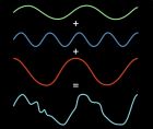
我们大家知道,傅立叶变换是我们很多科学领域的重要的数学工具。有人说没有傅立叶变换就没有我们现代科学一些新分支或者很多学科就可能不太完善,我觉得这句话一点没有错。我们在地球物理的信号,无线电信号,现代的通讯技术、光学、声学甚至音乐中都大量应用傅立叶变换,尤其是离散的傅立叶变换。美国麻省理工学院(MIT)最近在她的网站主页上用非数学的语言给普通民众大谈离散傅立叶变换(DFT),这篇文章很通俗,推荐给大家共享,希望大家多多讨论。 网站链接: http://web.mit.edu/newsoffice/2009/explained-fourier.html Explained: The Discrete Fourier Transform The theories of an early-19th-century French mathematician have emerged from obscurity to become part of the basic language of engineering. Larry Hardesty, MIT News Office November 25, 2009 Science and technology journalists pride themselves on the ability to explain complicated ideas in accessible ways, but there are some technical principles that we encounter so often in our reporting that paraphrasing them or writing around them begins to feel like missing a big part of the story. So in a new series of articles called Explained, MIT News Office staff will explain some of the core ideas in the areas they cover, as reference points for future reporting on MIT research. In 1811, Joseph Fourier, the 43-year-old prefect of the French district of Isre, entered a competition in heat research sponsored by the French Academy of Sciences. The paper he submitted described a novel analytical technique that we today call the Fourier transform, and it won the competition; but the prize jury declined to publish it, criticizing the sloppiness of Fouriers reasoning. According to Jean-Pierre Kahane, a French mathematician and current member of the academy, as late as the early 1970s, Fouriers name still didnt turn up in the major French encyclopedia the Encyclopdia Universalis. Now, however, his name is everywhere. The Fourier transform is a way to decompose a signal into its constituent frequencies, and versions of it are used to generate and filter cell-phone and Wi-Fi transmissions, to compress audio, image, and video files so that they take up less bandwidth, and to solve differential equations, among other things. Its so ubiquitous that you dont really study the Fourier transform for what it is, says Laurent Demanet, an assistant professor of applied mathematics at MIT. You take a class in signal processing, and there it is. You dont have any choice. The Fourier transform comes in three varieties: the plain old Fourier transform, the Fourier series, and the discrete Fourier transform. But its the discrete Fourier transform, or DFT, that accounts for the Fourier revival. In 1965, the computer scientists James Cooley and John Tukey described an algorithm called the fast Fourier transform, which made it much easier to calculate DFTs on a computer. All of a sudden, the DFT became a practical way to process digital signals. Summing together only three discrete frequencies can produce a much more erratic composite. The Fourier transform provides a way to decompose signals into their constituent frequencies. To get a sense of what the DFT does, consider an MP3 player plugged into a loudspeaker. The MP3 player sends the speaker audio information as fluctuations in the voltage of an electrical signal. Those fluctuations cause the speaker drum to vibrate, which in turn causes air particles to move, producing sound. An audio signals fluctuations over time can be depicted as a graph: the x-axis is time, and the y-axis is the voltage of the electrical signal, or perhaps the movement of the speaker drum or air particles. Either way, the signal ends up looking like an erratic wavelike squiggle. But when you listen to the sound produced from that squiggle, you can clearly distinguish all the instruments in a symphony orchestra, playing discrete notes at the same time. Thats because the erratic squiggle is, effectively, the sum of a number of much more regular squiggles, which represent different frequencies of sound. Frequency just means the rate at which air molecules go back and forth, or a voltage fluctuates, and it can be represented as the rate at which a regular squiggle goes up and down. When you add two frequencies together, the resulting squiggle goes up where both the component frequencies go up, goes down where they both go down, and does something in between where theyre going in different directions. The DFT does mathematically what the human ear does physically: decompose a signal into its component frequencies. Unlike the analog signal from, say, a record player, the digital signal from an MP3 player is just a series of numbers, representing very short samples of a real-world sound: CD-quality digital audio recording, for instance, collects 44,100 samples a second. If you extract some number of consecutive values from a digital signal 8, or 128, or 1,000 the DFT represents them as the weighted sum of an equivalent number of frequencies. (Weighted just means that some of the frequencies count more than others toward the total.) The application of the DFT to wireless technologies is fairly straightforward: the ability to break a signal into its constituent frequencies lets cell-phone towers, for instance, disentangle transmissions from different users, allowing more of them to share the air. The application to data compression is less intuitive. But if you extract an eight-by-eight block of pixels from an image, each row or column is simply a sequence of eight numbers like a digital signal with eight samples. The whole block can thus be represented as the weighted sum of 64 frequencies. If theres little variation in color across the block, the weights of most of those frequencies will be zero or near zero. Throwing out the frequencies with low weights allows the block to be represented with fewer bits but little loss of fidelity. Demanet points out that the DFT has plenty of other applications, in areas like spectroscopy, magnetic resonance imaging, and quantum computing. But ultimately, he says, Its hard to explain what sort of impact Fouriers had, because the Fourier transform is such a fundamental concept that by now, its part of the language.
 标签: 傅立叶变换
![[转载]傅立叶变换](http://image.sciencenet.cn/album/201302/26/22092916zfa81gawa35mq1.jpg.thumb.jpg)