原载 http://blog.sina.com.cn/s/blog_729a92140102wc7i.html 本短文用“实变换时”表明:限于Tpwp中,特别地假定被处理信号和滤波器冲激响应,都是实数序列。不管Tpwp之外的变换,因为使用DFT的条件和方法不一样。这里,不涉及人们从文献中可能见到的奇偶时间点序列分组、FIR以及时间延迟之类的问题,给定的一个被处理序列x和滤波器序列F(高通或低通),必须靠“移位方向参量为空值”另外指明它们都是频域区间 的结果仍等于v。 以博文《减少小波包变换的DFT算法模式中的DFT的次数和点数》(2015-10-26)为基础,减少了部分复数乘法,但是,新增了复共轭、向量倒序的处理内容,改变了那里的“频域数据重复”与频域的乘积运算的顺序。 用这两个函数子程序,覆盖掉以前用的旧子程序,重新运行博文《冗余小波包合成以及降噪试验和能量守恒定标》(2015-12-27)的最后三个降噪实验。可见在Scilab-5.3.3的命令窗中显示了相同的数字(format(‘v’,10) 格式)结果。但是,有些遗憾,没有见到实验的总耗时量明显减少,甚至反而可见高达百分之十几的增加,这可能与引入的其它处理以及系统工作平台中整体的解释、管理等有关。据此类经验,比较算法的性能时,居士希望尽量交代清楚方案、条件、环境。 新浪赛特居士SciteJushi-2016-05-13。 图片 1. 减少了紧凑DFT算法模式中实变换时的频域乘法的次数的程序段 附 . 最近,搜索小波的最新研究进展,在《百度百科》中,注意到了中国已有研究成果“比小波分析创始人Mallat提出的著名Mallat算法快一个数量级以上,而且效果和质量远优于Mallat算法”。看到这很振奋又好奇,然而还未搜到演示资料或方法细述,故特将其复制为留念于下。原来,还有了国际小波分析应用研究中心。虽然,姓名,是居士在博客中多次提到(因个人认为,翻译得已很不错)的小波名著“十讲”的译者,也是前面(2016-04-20)的实变换的滤波器构造中曾用过那篇中文参考文献的作者。但是,居士真不记得当年离开小波的研究时,对这个姓名已有印象,实际上,除去博文已明确提到的部分,至今仍几乎未知其具体研究(注意,在此无褒贬之意)。 : 李建平(电子科技大学教授) 简介?编辑 1986年获重庆大学应用数学理学学士,1989年获西安交通大学软件工程、计算数学双硕士学位,1998年获重庆大学计算机科学理论工学博士学位,1999年至2001年到香港浸会大学做博士后研究,2002年至2003年到法国普罗旺斯大学做访问学者,2005年至2006年到加拿大圭尔夫大学、多伦多大学做访问学者. 教学情况 现为电子科技大学计算机科学与工程学院、示范性软件学院副院长,国际小波分析应用研究中心主任,国际学术进展 International Progress on Wavelet Active Media Technology and Information Processing主编,国际学术期刊International Journal of Wavelet Multiresolution and Information Processing副主编,兼任国家科学技术奖励评审委员、国家自然科学基金项目评审委员、中华人民共和国公安部技术顾问等十几个学术、社会职务,是2004年国际计算机学术大会、第三届国际小波分析及其应用学术大会(ICWAA)、第二届智能体媒介技术国际学术大会(ICAMT)主席,是国际上小波分析与信息处理研究领域十分活跃的知名专家。 科研情况 他在国际上独立提出并系统建立了“小波变换的加速方法”、“矢量积小波变换理论”、“基于小波分析的电子签名系统”等系列理论与方法,该理论比小波分析创始人 Mallat提出的著名Mallat算法快一个数量级以上,而且效果和质量远优于Mallat算法,这为小波理论在信号处理、信息分析等许多方面的应用提供了先进的算法,为小波分析的实时处理和产品化提供了理论基础,为小波分析开辟了广阔的应用前景。他在国际上首次提出“基于‘三大特征’(机器特征、文档特征、人体特征)的信息最安全传输的模型与方法”,为当今研究热点的网络与信息安全做出了重要贡献。他先后主持国家863高技术项目、国家自然科学基金项目等30项。他在国内外著名学术期刊上发表重要论文150篇,被国际三大检索机构SCI、EI、ISTP等检索收录论文48篇,出版学术专著15部,其中2部被多次修订重印。他主持研制的“小波指纹加密系统”、“分布式网络监控系统”等高技术产品产生了广泛的经济效益和社会影响
原载 http://blog.sina.com.cn/s/blog_729a92140102vz7w.html 由于某些原因,人们在应用实践中,常未明确考虑基于连续时间小波基函数的被处理数据初始化问题,或无交代,甚至有人误以为Mallat算法就已解决了这一问题。有研究者,对此状况,持较严厉的批评态度,于是有“小波罪恶(wavelet crime)”之说,如图片1的顶部所示。 把离散变换和连续时间信号联系起来,可以更好地理解和开拓应用,但这样常不得不接受近似处理。在与Mallat算法有关的小波变换中,过渡联系的麻烦,表现得尤其突出,难被消除。严格地说,在很多实践中,紧支集连续时间小波基函数,还不算真有用。 习惯于傅立叶分析时,可能想,用矩形窗截取FIR低通滤波器序列的傅立叶变换的一个周期,然后利用频谱的伸缩以获得不同的低通带宽度,就得意味着不同分辨率的子空间簇。然而实际上,在Mallat等的连续时间能量有限信号空间的多分辨分析理论中,尺度函数以及嵌套子空间列,有非直观的特殊的定义方式。人们常难由FIR滤波器组用闭式表达连续时间基函数,只知在极限意义上存在,一个具有某些性质的连续时间尺度函数和小波函数系。 即使,可用解析式表示被处理信号,也不一定容易计算出它与某个紧支集基本函数的平移系的内积,更何况,实际应用中常常只知离散序列 (名著“十讲”第五章后的注释 12,是研究初始化滤波的引子), 难确定其对应的合适函数子空间。这个内积,是连续时间基函数的应用解释的严密性的关键,而也反使数字频率与模拟信号物理频率的精确联系变得麻烦。 如果什么都已知的话,也许 人们 就不需离散小波变换,来做压缩或降噪等事情了。 见到Matlab小波工具箱通过数字计算画个小波函数曲线时,也不清楚其中局部扭结小尖峰,正是好的性质的体现,还是有了较多数字误差。 居士脱离连续时间,直接讨论离散小波包变换,可以使计算理论更独立严谨。这正如,离散傅立叶变换及其快速算法,不必依赖于,连续时间和连续频率概念。由离散时间滤波器组,进入某些函数空间,在其中做理论分析等,是其它的故事。不同的部分,各有价值。 某些问题还未解决好,或未被意识到,或者论述行文失误,都是研发中较常见的事,不意味着“犯罪或邪恶”。这正如,不能说,应用傅立叶变换或Shannon采样定理时的不都定量的近似,是“违法”行为。现代的傅立叶变换理论,已包括很多部分,在数字计算中实际常用的是FFT。各部分连接的关键基础,在长时间的大量文献中 , 同样可能有“不尽人意”之处。当然,批评与自我批评,有事说事,努力解决问题,这是正道。 在傅立叶让他的级数出世后,人们用了相当长的时间,理清傅立叶级数的收敛性问题。 图片1.中关于采样定理的描述,取于国内外的著名教科书或著作,并不是研发初学者之作。 看起来,不算“明确而精辟”。 为什么不用开区间,表示信号的频谱?直观地看:采样使频谱周期延拓时,闭区间有重叠点,使“离散谱”混叠、消失、或不能区分两个边界频率;而且,理想滤波器的频响,在边界频率处不连续,使人感到,不确定、不安全、宜避开。开区间,至少从形式上就排除了麻烦:在边界频率上的正弦信号一个周期内,正好都采到零。 为什么不用半开半闭区间,表示信号的频谱?直观地看:频谱周期延拓时,可无重叠点,也包括了整个频率轴,更像是在频谱的采样离散化时单个周期的两端点中只取一侧。 早期的采样定理中的信号及其傅立叶变换,到底需要什么严格条件? 维基百科,并不排除,定理适用于频率在边界以内的正弦信号(如文后附1.)。“教育部研究生工作办公室推荐研究生教学用书”《数字信号处理》,有专节讨论正弦信号抽样的问题。更一般地讲,定理要面对离散频率成分的问题。 绝对可积函数的傅立叶积分变换,或连续频谱函数,不适用于正弦波。像Dr.Daubechies那样,把带限信号集,视为能量有限 (无穷时间) 信号空间的子空间,陈述采样定理时,也排除了正弦函数等功率有限而能量无限的周期信号。 使用冲激函数串来推演采样定理,这意味着引入了广义函数的傅立叶变换。统一表达了离散谱线和连续区间上的频谱之后,定理就包括了正弦函数。 现在相信,实际信号都是能量有限的,不存在无始无终的永动机式的精确单频率运动过程,人们天天做的采样、数-模转换、滤波都是现实的。然而,信号分析实验中常用的三角函数模型和采样定理中的sinc插值重建函数,都不是物理可实现的。 即使,认为现实中能记录的信号,都既是时限的也是带限的,也不都很精确每个实际问题中的误差,一般也不随Slepian等研究“时-频限”。很多时候,也未必明确所谓的冲激函数串的理想化抽象近似的量度。 Shannon采样理论,用sinc函数做 理想 插值重建(Whittaker–Shannon interpolation formula),违背因果律。很强调了带限,削弱了对现实时限的注意。实际上,采样率变化了,那么,某给定时间区间内的重建信号,受该区间外的样本点影响的程度,也就不同了。假如对插值函数做截断近似,则还需要兼顾函数值的量化误差。 至此,容易注意到,过采样的采样率很高时,可以认为很多“插值函数、重建基函数”都可“更近似于冲激函数”,其差别减小了。这样,使用多分辨分析子空间的小波变换的初始化时,误差也可能减小。 记得当年老师说,凭经验,实用电路中,采样频率一般大于信号成分的最高频率的2.5倍,因为低通模拟滤波器的过渡带不是理想的。田边顽童,不识定理,更无非均匀采样理论,而可能用小石子或谷粒拼出些自以为像人头的图案,指指点点,叫这个狗娃,称那个胖仔。 新浪赛特居士SciteJushi-2015-11-22。 图片 1.小波罪恶之说与采样定理的表述 附 1:Wikipedia中的采样定理(Nyquist–Shannon sampling theorem) 部分的摘录 Sampling is the process of converting a signal (for example, a function of continuous time and/or space) into a numeric sequence (a function of discrete time and/or space). Shannon's version of the theorem states: If a function x(t) contains no frequencies higher than B hertz, it is completely determined by giving its ordinates at a series of points spaced 1/(2 B ) seconds apart. A sufficient sample-rate is therefore 2 B samples/second, or anything larger. Equivalently, for a given sample rate f s , perfect reconstruction is guaranteed possible for a bandlimit B ≤ f s /2. When the bandlimit is too high (or there is no bandlimit), the reconstruction exhibits imperfections known as aliasing. Modern statements of the theorem are sometimes careful to explicitly state that x ( t ) must contain no sinusoidal component at exactly frequency B , or that B must be strictly less than ½ the sample rate. The two thresholds, 2 B and f s /2 are respectively called the Nyquist rate and Nyquist frequency . And respectively, they are attributes of x ( t ) and of the sampling equipment. The condition described by these inequalities is called the Nyquist criterion , or sometimes the Raabe condition . The theorem is also applicable to functions of other domains, such as space, in the case of a digitized image. The only change, in the case of other domains, is the units of measure applied to t , f s , and B .
原载 http://blog.sina.com.cn/s/blog_729a92140102vngc.html 此前,在讨论小包分解与合成计算时,用变量Wp.RightShift控制生成基向量组时移位的左、右方向两种选择。在Tpwp的函数子程序( 如图片1.的右上角所示 )中,添加几个语句 (即if isempty(Right_Shift)…end部分),就直接增设了DFT(离散傅立叶变换)算法模式。用工作平台自带的计算DFT和逆变换IDFT的函数fft和ifft。因为,不必究等效地实现了以前的某部分计算,也不强调其对应外部的反转、移位关系等,所以居士列其为小波包变换的另一种设置选项。 虽然,使用的仍都是已知的时域尺度序列数据,但是,Tpwp明显不排除:直接解算和构造滤波器组的“离散频率”序列。 反复用“随机设置”一词,针对深奥呆板的形象。在不同的编程语言环境中,也不必精确一一对等地,实现那些所谓的设置。不证明某个选择特别正当,但是,始终以Matlab-R2011a工具箱中“实数域的普通离散小波变换”的“标准模式和算法”的重建误差为参照,表明它们都可行。某个选择可能只构成另一些设置的等效计算,也可能意味着用了不同的小波包基,可能使“小波包林”扩张了。 可用快速傅立(或付、里)叶变换FFT计算卷积,这在信号处理教科书中是常识。在小波变换理论与应用文献中,离散信号的分解与重构,都使用了线性卷积滤波器。自然地,很早就有研究论文,试用FFT来计算离散小波变换。本短文更表明, Tpwp的演绎机制的特点,使增设DFT算法模式,尤其简捷。 小波工具箱中的“数据边界延拓模式”以及Wavelab850中的“延拓后用函数filter”的方法,把一个圆卷积问题,也反而转化成了线性卷积来处理。然而,Tpwp理论把线性卷积问题首先周期化,再推演有限维酉空间的小波包分割与覆盖,所以其计算与FFT更靠近。 对被分解序列做FFT,再与基向量的频域序列F相乘,把乘积序列的逆傅立叶变换IFFT后(注意,也已算出要抛弃的部分)的下抽象样值,作为分解结果。对输入序列补插零值后,做FFT,再与基向量的频域序列相乘,把乘积序列的IFFT输出,作为合成结果。 验证方法的程序之一, PwpRandComplexFFT.m ,由《随机设置小波包变换的强迫复数化的测试》( 2014-11-25)中的 PwpRandComplex.m 改写而成。从图片1.的右下角,可见主要改变,在于插入了条件语句 if abs(Wp.RightShift)5e5, % about 60% tests Wp.RightShift= =TpwpGHfft(... phcoef,pgcoef,rphcoef,rpgcoef,Wp.DatL,Wp.DecL); end % FFT, on all the basis vectors 其中,把 Wp.RightShift,强行改为空矩阵作为标志,指示按 DFT算法模式使用基向量组,否者,仍用旧移位方式;子程序TpwpGHfft用FFT,预先将基本基向量组变换到频域。这是正确使用DFT算法模式,需要做的两件事情。其余程序语句,与 PwpRandComplex.m比, 不变。 一般说来,DFT要求整个处理系统用复数域,而且,函数子程序集,要能兼容控制复数化共轭滤波器组。若在降噪以及预置基的函数子程序中增加TpwpGHfft控制,那么,在降噪和分类识别等试验中,就可使用DFT算法模式了。新函数子程序包TpwpSubs.bin,比旧包大了11KB;TpwpSubs_E01.bin,约增大了1KB。仍用完全安装的Scilab-5.3.3制作,不从互联网下载任何工具箱和优化库文件,也无需用户库。 重编译 子程序集时,尽量少改,即使对于曾测到 rigrsure应用中的被零除的状况也保留(系数加权时可滤掉)。 用高级语言 编 程,且一般做“概念性的、演示性的”实现,不必需移位、数据寻址等的效率优化。 但是,顺便,遵循 Matlab编辑器的建议,在某些子程序中,把原未经初始化然而在循环语句中却需不断改变大小的向量,首先初始化了,这可能影响旧试验的 总耗时量。 生成图片1.中的曲线图,总的耗时约为1955秒,验证了兼容性、双向重建性质、双向保内性质。使用了128组尺度序列、2560组随机复数化滤波器、2560次深度为8的完整树小波包分解、5120次约束树分解、10240次小波包合成。每次分解的复随机信号以及用于合成的复随机系数序列的长度,随机地取为1、3、5、7、9或11与256的乘积。其中约百分之六十,用到了DFT算法模式。FFTW库的设置为estimate,这是Matlab默认的(其帮助文档说“The default method is estimate…If you set the method to 'estimate', the FFTW library does not use run-time tuning to select the algorithms. The resulting algorithms might not be optimal.”)。 用同样的输入参数,运行原 PwpRandComplex.m ,即无 DFT算法模式时,总的耗时约为:4381秒。 在《续用小规模人工神经网络试做个对留数不敏感的分类器》(2015-04-02)所用的测验程序WpdcNN1.m中,把参数Wp.RightShift=1改为Wp.RightShift= ,即将“右移位方式”改为“DFT算法模式”后,再运行,可见降噪性能非常接近然而可节约约百分之二十五的时间。 被处理信号和滤波器组都是实数值序列时,如果不引入DFT,那么分解与合成的结果,也都自动为实数值。然而,经复变换过程后,数字误差可能引入复数,尽管虚部可以很小。虚部值依赖于机器系统精度,也与实现傅里叶变换的子程序对对称性、虚部、实数性等的识别和控制有关(据居士已有经验,Matlab做得很好),这可能使兼容性问题和应用复杂化,总的处理时间也可能反而增加。这时,就不宜选DFT算法模式 。 涉及fft和ifft时,不用Scilab-5.5.0。若用,就除去其FFTW模块的库文件libfftw3-3.dll (资源管理器显示,2311KB, 2013-8-30)后,再重启动,使用默认的标准FFT (standard fft by default),才可实现类似于图片1.中那样的测验。这个文件,约为在5.3.3版中旧库(805KB, 2009-10-29)的3倍大,可能有了相当充分的优化控制,而与居士所用的机器系统难兼容。 新浪赛特居士SciteJushi-2015-05-13。 图片 1.DFT算法模式以及用强迫复数化滤波器组的测证结果(Matlab版)
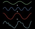
据MIT新闻网站报道,MIT的科学家研究出比FFT更快的傅立叶变换算法。 The Fourier transform is one of the most fundamental concepts in the information sciences. It’s a method for representing an irregular signal — such as the voltage fluctuations in the wire that connects an MP3 player to a loudspeaker — as a combination of pure frequencies. It’s universal in signal processing, but it can also be used to compress image and audio files, solve differential equations and price stock options, among other things. The reason the Fourier transform is so prevalent is an algorithm called the fast Fourier transform (FFT), devised in the mid-1960s, which made it practical to calculate Fourier transforms on the fly. Ever since the FFT was proposed, however, people have wondered whether an even faster algorithm could be found. At the Association for Computing Machinery’s Symposium on Discrete Algorithms (SODA) this week, a group of MIT researchers will present a new algorithm that, in a large range of practically important cases, improves on the fast Fourier transform. Under some circumstances, the improvement can be dramatic — a tenfold increase in speed. The new algorithm could be particularly useful for image compression, enabling, say, smartphones to wirelessly transmit large video files without draining their batteries or consuming their monthly bandwidth allotments. Like the FFT, the new algorithm works on digital signals. A digital signal is just a series of numbers — discrete samples of an analog signal, such as the sound of a musical instrument. The FFT takes a digital signal containing a certain number of samples and expresses it as the weighted sum of an equivalent number of frequencies. “Weighted” means that some of those frequencies count more toward the total than others. Indeed, many of the frequencies may have such low weights that they can be safely disregarded. That’s why the Fourier transform is useful for compression. An eight-by-eight block of pixels can be thought of as a 64-sample signal, and thus as the sum of 64 different frequencies. But as the researchers point out in their new paper, empirical studies show that on average, 57 of those frequencies can be discarded with minimal loss of image quality. Heavyweight division Signals whose Fourier transforms include a relatively small number of heavily weighted frequencies are called “sparse.” The new algorithm determines the weights of a signal’s most heavily weighted frequencies; the sparser the signal, the greater the speedup the algorithm provides. Indeed, if the signal is sparse enough, the algorithm can simply sample it randomly rather than reading it in its entirety. “In nature, most of the normal signals are sparse,” says Dina Katabi, one of the developers of the new algorithm. Consider, for instance, a recording of a piece of chamber music: The composite signal consists of only a few instruments each playing only one note at a time. A recording, on the other hand, of all possible instruments each playing all possible notes at once wouldn’t be sparse — but neither would it be a signal that anyone cares about. The new algorithm — which associate professor Katabi and professor Piotr Indyk, both of MIT’s Computer Science and Artificial Intelligence Laboratory (CSAIL), developed together with their students Eric Price and Haitham Hassanieh — relies on two key ideas. The first is to divide a signal into narrower slices of bandwidth, sized so that a slice will generally contain only one frequency with a heavy weight. In signal processing, the basic tool for isolating particular frequencies is a filter. But filters tend to have blurry boundaries: One range of frequencies will pass through the filter more or less intact; frequencies just outside that range will be somewhat attenuated; frequencies outside that range will be attenuated still more; and so on, until you reach the frequencies that are filtered out almost perfectly. If it so happens that the one frequency with a heavy weight is at the edge of the filter, however, it could end up so attenuated that it can’t be identified. So the researchers’ first contribution was to find a computationally efficient way to combine filters so that they overlap, ensuring that no frequencies inside the target range will be unduly attenuated, but that the boundaries between slices of spectrum are still fairly sharp. Zeroing in Once they’ve isolated a slice of spectrum, however, the researchers still have to identify the most heavily weighted frequency in that slice. In the SODA paper, they do this by repeatedly cutting the slice of spectrum into smaller pieces and keeping only those in which most of the signal power is concentrated. But in an as-yet-unpublished paper , they describe a much more efficient technique, which borrows a signal-processing strategy from 4G cellular networks. Frequencies are generally represented as up-and-down squiggles, but they can also be though of as oscillations; by sampling the same slice of bandwidth at different times, the researchers can determine where the dominant frequency is in its oscillatory cycle. Two University of Michigan researchers — Anna Gilbert, a professor of mathematics, and Martin Strauss, an associate professor of mathematics and of electrical engineering and computer science — had previously proposed an algorithm that improved on the FFT for very sparse signals. “Some of the previous work, including my own with Anna Gilbert and so on, would improve upon the fast Fourier transform algorithm, but only if the sparsity k” — the number of heavily weighted frequencies — “was considerably smaller than the input size n,” Strauss says. The MIT researchers’ algorithm, however, “greatly expands the number of circumstances where one can beat the traditional FFT,” Strauss says. “Even if that number k is starting to get close to n — to all of them being important — this algorithm still gives some improvement over FFT.” 引自: http://web.mit.edu/newsoffice/2012/faster-fourier-transforms-0118.html
 标签: FFT