不要说数据可视化的优点,以及为了展示给老板看。 本文参考维基百科: https://en.m.wikipedia.org/wiki/Anscombe%27s_quartet 下图是著名的安斯库母四重奏, 它们具有相同的统计值,但不同的x,y,然而结果用简单的线性回归建模却得到同样的结果,事实上,拟合的结果的准确性是值得商榷的,有的效果可以,有的却是错误的。 Property Value Accuracy Mean of x 9 exact Sample variance of x 样本方差 11 exact Mean of y 7.50 to 2 decimal places Sample variance of y 4.125 plus/minus 0.003 Correlation between x and y 0.816 to 3 decimal places Linear regression line y =3.00+0.500 x to 2 and 3 decimal places, respectively Coefficient of determination of the linear regression 线性回归的确定系数 0.67 to 2 decimal places 好好看看,第二个图和第四个图是不是直接错误,第三个图勉强算对,但不准确,有个离群值明显可以舍去。第一个图是正确的。 由此可见,在数据探索中,有必要进行简单的验证,查看数据是否可以用已有的模型,模型重要,但数据质量更重要。
IEEE Visualization Conference 2015 - Increasing Influence of Machine Learning IEEE Visualization Conference 2015 - Increasing Influence of Machine Learning ML Blog Team 11 Nov 2015 9:00 AM Comments 0 Likes This post is authored by Yiwen Sun, Data Scientist at Microsoft. I attended the IEEE Visualization Conference 2015 in Chicago recently and jotted down a few points related to machine learning. For those of you who are unfamiliar with this conference, it’s the largest annual gathering of practitioners, academics and researchers looking to make data visually understandable and usable. Conference paper talks are organized into three tracks: Visual Analytics Science and Technology (VAST), Information Visualization (InfoVis), and Scientific Visualization (SciVis). Co-located are three IEEE symposiums: Large Data Analysis and Visualization (LDAV), Visualization for Cyber Security (VizSec), and the very first Symposium of Visualization in Data Science (VDS). Over 1500 attendees participated this year, including leading companies in Business Intelligence and Advanced Analytics including Bloomberg, Google, IBM, Tableau, and, of course, Microsoft. One big impression I got is that ML and Data Visualization are getting coupled more tightly. Over half of the papers address ML techniques in their data processing step. For example, the best paper for VAST “ Reducing Snapshots to Points: A Visual Analytics Approach to Dynamic Network Exploration ” utilizes vectorization, normalization, and dimensionality reduction to project high-dimensional dynamic network data onto two dimensions, then visualize them using two juxtaposed views: one showing network snapshots and the other showing the evolution of the network. This enables users to differentiate regular, stable states from anomalies more easily. Below is a summary of ML techniques highlighted in four major application areas: In network or spatial data visualization, clustering and classification have been widely used to reduce clutter and identify regions of interest. For example, in the paper “ MobilityGraphs: Visual Analysis of Mass Mobility Dynamics via Spatio-Temporal Graphs and Clustering ”, hourly Twitter user movement data in Greater London area are spatially aggregated into regional clusters and color-coded by temporal clusters. (Image from Interactive Graphics Systems Group at Technical University of Darmstadt) For time-series data visualization, a big challenge is to present large dataset on the limited display space without over-plotting. An effective approach is to aggregate the data points into segments of time, and create a hierarchy of multi-focus zoomed line chart, as illustrated in the paper “ TimeNotes: A Study on Effective Chart Visualization and Interaction Techniques for Time-Series Data ” (Image from TimeNotes ) In textual data visualization, text mining techniques such as entity extraction, topic identification and sentiment analysis become essential. In the paper “ Exploring Evolving Media Discourse Through Event Cueing ”, multiple mining results, such as entities in Wordle, sentiment scores over timeline, are linked together to enable and enhance the analysis of media discourse. (Image from VADER Lab at Arizona State University) Anomaly detection, though not a standalone research area for visualization, has been studied by different research groups, to assist human judgement with automated analysis results. In “ Visualization and Analysis of Rotating Stall for Transonic Jet Engine Simulation ” the authors applied Grubbs’ test to identify outliers in blade passages as the early sign of turbine engine’s rotating stall. In “ TargetVue: visual analysis of anomalous user behaviors in online communication systems ”, TLOF (time-adaptive local outlier factor) model was used to identify sudden changes of user behaviors based on a set of features extracted for each user from the online communication data. The VAST Challenge was another highlight – this is an annual contest that began in 2006 and is designed to reflect real-world analytics challenges and encourage research into novel data processing, visualization and interaction methods. This year’s challenge was to analyze individual and group movement in an amusement park over a weekend which involves a criminal investigation. Popular languages used for data processing and ML were Python and R, both of which are currently supported by Azure Machine Learning . Overall, the conference was a great place to learn about the very latest in all things visualization, and to interact with experts in the domain. Yiwen 0 Comments 来源:http://blogs.technet.com/b/machinelearning/archive/2015/11/11/ieee-visualization-conference-2015-increasing-influence-of-machine-learning.aspx
LAB巡天全天的中性氢数据的可视化,对天球作了Mollweide投影,注意tvscl里Startx和Starty以及Xsize和Ysize对于图和坐标线的对齐有关键性的作用。目前程序表示的只是积分强度,尚没有转化为柱密度。 PRO processLAB fitsname='lab.fit';default file name deal,fitsname END PRO deal,fitsname ;Distance = 140.0; distance in units of parcec ;Distance = Distance*3.086d18; distance in units of cm head=headfits(fitsname);read the header of the fits file to a vector bw = fxpar(head,'BW'); band width freq = fxpar(head,'LINEFREQ'); central frequency nx = fxpar(head,'NAXIS1'); number of elements in the first dimension ny = fxpar(head,'NAXIS2'); nz = fxpar(head,'NAXIS3'); crvalx = fxpar(head,'CRVAL1'); reference value of the first dimension cdeltax = fxpar(head,'CDELT1'); increasement of the first dimension ; in units of degree, when calculate physical ; scale, must changed to arcdegree crpixx = fxpar(head,'CRPIX1'); reference position of the first dimension crvaly = fxpar(head,'CRVAL2'); cdeltay = fxpar(head,'CDELT2'); crpixy = fxpar(head,'CRPIX2'); crvalz = fxpar(head,'CRVAL3'); cdeltaz = fxpar(head,'CDELT3'); crpixz = fxpar(head,'CRPIX3'); bzero = fxpar(head,'BZERO'); bscale = fxpar(head,'BSCALE'); ;x=(findgen(nx)-crpixx)*cdeltax+crvalx; ;y=(findgen(ny)-crpixy)*cdeltay+crvaly; ;z=(findgen(nz)-crpixz)*cdeltaz+crvalz; ;area = Distance^2*(abs(cdeltax)/57.3)*(abs(cdeltay)/57.3) ; physical area per pixel ;print, area ;print, area*1.67d-24*weight/2d33 ;a=ptr_new(/allocate_heap) a=mrdfits(fitsname,0,/fscale); read the data cube to an array vchannel=abs(cdeltaz)/1.0e3 ; km/s ;a=readfits(fitsname) ;b=total(a,3); co-add the third dimension ;???? ;vchannel=bw/(nz*1.0d0)/freq*ckm; the velocity width corresponding to a channel ; units in km/s ;b=b*vchannel; intensity integrated with velocity (with unit: Jy km/s) ;???? ;b=b*vchannel; antenna temperature integrated with velocity (units K km/s) ;b=b*vchannel*1.93e3*nu^2*(1.0/3.0)/A; column density (units /cm^2) ; N_l=1.93*10^3*(g_l/g_u)*(nu^2/A_ul)\int T dv ;b=ptr_new(/allocate_heap) ;/for test ;*b=total(*a(1:100,1:100,*),3)*vchannel*1.93e3*nu^2*(1.0/3.0)/Alu*area*1.67d-24*weight/2d33 ; mass distribution in solar mass ;for test b=total(a,3) ;b=a bad=where(finite(b) eq 0, count) if(count gt 0) then b(bad)=0.0 ;b=(b+abs(b))/2.0 ;b=b*vchannel*1.93e3*1.42^2/4.65e-17*(4.0/3.0) b=b*vchannel*(4.0/3.0) b=b/1.0e3 print,max(a) maxb=max(b) print,maxb print,(min(a)-bzero)/bscale colors=200 clrtablelength=colors ;color_array=findgen(256L) ;clevs=findgen(256L) LoadCT, 5, NColors=colors, Bottom=1, /Silent device,decompose=0 ;loadct,5 ;tvlct, , , ,1 latmin=-90 latmax=90 lonmin=-180 lonmax=180 ;position = position = margin=0.12 ;margin=0.5 wall=0.03 xsize=18.8 aa=xsize/8.8-(margin+wall) bb=aa*2d/(1+sqrt(5)) ysize=(margin+bb+wall+bb+wall)*6.8 ;================================================ set_plot,'PS' filename=fitsname+'_TV.eps' ; set the file name of the output ps file device,file=filename,/ENCAPSULATED,/COLOR, BITS=8;,xsize=xsize,ysize=ysize ;tvscl,c(1:1000,1:1000) ;tvscl,b map_set,0,0,/MOLLWEIDE,/ISOTROPIC,/HORIZON,/GRID result=map_image(b,Startx,Starty,Xsize,Ysize,compress=1,LATMIN=latmin,$ LONMIN=lonmin,LATMAX=latmax,LONMAX=lonmax,scale=0.1) result=bytscl(result,Min=0.01) tvscl,result,Startx,Starty,XSIZE=Xsize,YSIZE=Ysize ;tvscl,result ;print,Startx,Starty ;TVimage,BytScl(result, Top=99) ;lons=indgen(360/20+1)*20*(-1)+180 lons=indgen(360/45+1)*45-180 lonnames=strtrim(-lons) ;print,lonnames ;map_grid,latdel=10,londel=20,lons=lons,color=0.30*!d.n_colors,/LABEL,/HORIZON map_grid,latdel=20,londel=20,lonnames=lonnames,lons=lons,$ color=0.80*!d.n_colors,charthick=2,glinethick=3,/LABEL,/HORIZON ;;colorbar,ncolors=256,POSITION= ;ticks=strtrim(sindgen((clrtablelength/5+1)*5)-(clrtablelength/2),2) ;Colorbar, Range= , Divisions=10, $ ;Minor=5, NColors=colors, Bottom=1, $ ;Position=position,Charsize=1,ticknames=tickes timesstr=textoidl('\times 10^{4} K\cdot km/s') Colorbar, Range= , Divisions=10, $ Minor=5, NColors=colors, Bottom=1, $ Position=position,Charsize=1,title=timesstr ;xyouts, 90, 180,timesstr,charsize=1.5,charthick=1.5,color=0;.80*!d.n_colors ;tlb=widget_base() ;labeltext='shit' ;label=widget_label(tlb,value=labeltext,ysize=40,units=0) ;widget_control,tlb,/realize device,/CLOSE ;================================================ ;spectra of each pixel ;print,"enter the coordinate of the pixel you need:" ;print,"ix(1 ~",nx12,")"," iy(1 ~",ny12,")"; ;read,ix,iy; ;plot,z,a ; ;find peak ;(pixel number - crpix)*cdelta+crval END
 标签: 数据可视化