分子云中的湍流激荡 中国科学院国家天文台 钱磊 (本文发表于国家天文台公众号,) “When I meet God, I am going to ask him two questions: Why relativity? And why turbulence? I really believe he will have an answer for the first.” —— Werner Heisenberg 摘要:湍流作为经典物理中的重要现象,其规律至今没有被完全理解。湍流普遍存在,和生活、工作和科学研究有紧密联系。凡是和流体有关的地方,很多时候都绕不开湍流。湍流虽乱,却“乱而有序”,这也是吸引众多科学家对其进行研究的原因。分子云作为恒星育婴所,湍流在其中起到了重要作用。湍流不仅可能解释了恒星形成的种子的来源,也可以给出分子云性质的一些信息。我们虽然已经了解了分子云中湍流的一些规律,但我们仅仅看到了冰山一角,还有很多未知等待我们探索。 湍流简述 湍流(turbulence)是经典物理学中最重要的未解决问题之一。公认关于湍流的文字和图像描述可以追溯到达芬奇的著作(图1)。按字面意思,湍流是急流的意思,抓住了湍流的一个特征。湍流以前也称为紊流,字面意思是乱流,也抓住了湍流的一个特征。从表象上看,紊流这个名称更符合实际,而湍流这个名称更加深刻——我们观察到,当流动速度变大到一定程度,就会产生湍流。 图1. 达芬奇著作中描绘的湍流。(来源:Wikipedia) 湍流虽乱,但一方面对我们的工作生活影响很大,另一方面乱中有序,吸引了众多学者对其进行研究。朗道 和钱德拉塞卡 这样的物理和天体物理大家都尝试提出湍流理论。虽然他们的理论有严谨的形式,但最终还是没能正确、完整地描述湍流。 图2. 层流。(来源:《An Album of Fluid Motion》) 在流动速度较小的时候,我们观察到流动是平稳有序的。如果对流体进行部分染色,我们可以看到流动时明显分层的,这种流动称为层流(laminar flow,图2)。当流速增大到一定程度,我们观察到,层流中会出现旋涡,流动变得杂乱无章,看不到明显的分层,这种流动称为湍流。注意到,我们说流动增大到“一定程度”,就会出现湍流,为什么不给个明确的判据,而要用“一定程度”这种模糊的词?因为我们不知道这个判据是什么。虽然一直以来,我们用雷诺数(Reynolds number)$Re\\equiv \\frac{uL}{\\nu}$(代表惯性力和粘滞力的比值)的大小作为层流向湍流转捩的判据,但是我们并不能给出一个精确的数值,大于这个值,湍流就能发生。事实上,虽然目前公认纳维-斯托克斯方程可以完整描述湍流,但是这个方程的一般解的存在性作为克雷数学研究所的七个千禧年问题之一还未得到解决。 虽然湍流的基本理论碰到了很大困难,但湍流的实验、观测、统计、唯象描述以及数值模拟取得了很多进展。其中,最重要和最著名的结论大概就是苏联数学家柯尔莫哥洛夫在1941年给出的不可压缩湍流(即密度不变、速度场散度为零的湍流)的指数为-5/3的幂律能谱 ,$E_k\\propto k^{-\\frac{5}{3}}$,对应的速度和尺度的关系为$v\\propto l^{\\frac{1}{3}}$。这个幂律是对于三维各向同性情形,假设能量在一个较大尺度注入,以固定的速率沿尺度从大到小级联传递,在一个较小尺度耗散而得到的。此后的研究给出了其他一些幂律关系,但公认的鼻祖还是柯尔莫哥洛夫的-5/3幂律。对于可压缩湍流,没有简单的规律,但有文献指出,将密度和速度结合起来仍然可以给出一个幂律,$\\rho v\\propto l^{\\frac{1}{3}}$。 不可压缩湍流的简洁性使其在理论和实验研究中有重要价值。而在实际应用,尤其是天体物理学中,可压缩湍流才更符合实际情况。 分子云中的湍流 湍流对于分子云有重要意义。(可压缩)湍流造成的密度涨落产生了密度较高的区域,这些区域可能是云核和恒星形成的种子。观测中发现,只有几十分之一的气体形成了恒星,因为致密气体的比例只有那么高。这些致密气体的形成可能和湍流有密切关系。 观测发现,分子云的谱线宽度通常比热致展宽要大很多。通常认为是分子云中的湍流导致了这种展宽。对众多分子云的观测也发现了分子云线宽$\\Delta v$和尺度 L 之间的一个有趣而重要的关系 ,称为拉尔森关系( Larson’s law ),以其发现者命名。拉尔森最早发现$\\Delta v\\propto l^{0.38}$,幂指数 0.38 接近 1/3 ,大家认为这可能说明分子云中的湍流是不可压缩的。但是后来更多的观测表明$\\Delta v\\propto l^{0.5}$ ,这表明分子云中的湍流是可压缩的。根据线宽估计,分子云中的湍流马赫数可以达到 10 ,对于这么大的马赫数,湍流应该是可压缩的。 由于动态范围(观测区域大小和望远镜最小可分辨尺度之比)有限,早期拉尔森关系的研究无法对单块分子云进行仔细研究,而是对一个分子云样本进行统计。随着观测数据的积累,已经对近邻的一些分子云,例如金牛座分子云、蛇夫座分子云,进行了成图观测,动态范围达到了 2000 ,这使得可以对这些分子云进行“拉尔森关系”的研究,即研究不同尺度上的速度弥散。要进行这项研究,还需要找到流场的标记物。曾经,人们通过一次偶然投放到海洋中的橡胶鸭子对洋流进行了标记(图 3 )。在分子云中,我们用的是云核。因为是用云核测量速度弥散,所以这种方法叫做云核速度弥散( CVD )。 图 3. 掉入大海中的橡皮鸭子可以用来标记洋流。(来源:geogarage.com) 我们的研究发现,对于金牛座分子云,速度弥散和尺度的关系符合拉尔森关系 ( Qian, Li, Goldsmith 2012, ApJ, 760, 147; http://nao.cas.cn/xwzx/kydt/201210/t20121017_3659876.html ),即$\\Delta v\\propto l^{0.5}$(但仔细分析可以发现不同尺度似乎有不同的幂指数,背后的原因还值得探讨)。而对于蛇夫座分子云,速度弥散似乎和尺度无关。这是因为天文观测不可避免地受到投影效应的影响,我们观测到的尺度都是投影到天球上的“二维投影尺度”,而湍流的幂律关系中的尺度是三维尺度,当分子云厚度较小时,三维尺度和二维投影尺度相差不大,而当分子云厚度较大时,二者相差很大。所以一个自然的推论是,如果我们在一块分子云中看到速度弥散和二维投影尺度之间满足拉尔森关系,则这块分子云可能是薄的!金牛座分子云(图 4 )可能就是这样一块薄的分子云 ( Qian et al. 2015, ApJ, 811, 71; http://nao.cas.cn/xwzx/kydt/201509/t20150909_4422532.html ),我们对金牛座分子云中 B213 区域厚度的测量也证实了这一点 (Li, Goldsmith 2012, ApJ, 756, 12) 。此外,由于分子云可能在一个维度受到压缩,并且存在磁场,分子云中的湍流可能存在各向异性。这可以通过速度弥散沿不同方向的变化趋势进行研究。 图 4. 金牛座分子云。(来源:国家天文台) 分子云中的超声速湍流给天文学家造成了很大困扰,因为理论上湍流能量应该很快就耗散掉了。我们能观测到湍流普遍存在,说明一定存在某种能量注入机制。已经提出的可能的能量注入机制包括星系盘的较差转动、引力塌缩以及恒星演化过程中的反馈(例如,星风和外流)。我们的研究发现,恒星演化的反馈过程提供的能量足以维持分子云中的湍流 (Li et al. 2015, ApJS, 219, 20; http://nao.cas.cn/xwzx/kydt/201511/t20151104_4453609.html ) ,但湍流能量注入机制到底为何,还有待进一步研究。一头一尾,说了能量来源,再说说能量的去处,有研究指出,可以通过观测中阶 CO 转动跃迁看到湍流的耗散 。最近,我们也用云核速度弥散方法估计了金牛座分子云中的湍流耗散率,得到的结果和用数值模拟得到的半解析公式估算的结果一致 (Qian et al. 2018, ApJ, 864, 116) 。 结语 自达芬奇描述湍流以来已经有近五百年了,自柯尔莫哥洛夫提出-5/3幂律能谱也已经有近八十年了。对湍流的研究仍然处于博物学阶段和唯象学阶段,仍然在收集湍流的标本,寻找这些标本的统计规律,提出湍流的统计理论。要从根本上理解湍流,还需要在基础理论中进行探索,至少首先回答纳维-斯托克斯方程一般解的存在性问题。未来,在基础理论没有大的进展的情况下,最有希望依赖的可能还是不断变得强大的计算机。 另一方面,在分子云的观测中,仍然存在天球投影造成信息不全的问题。精确测量分子云的三维结构和三维速度场是进一步了解分子云中湍流的必由之路。 参考文献 L. D. Landau, E. M. Lifshitz 1987, Fluid Mechanics. S. Chandrasekhar 1954, The Theory of Turbulence. A. Kolmogorov 1941, Doklady Akademiia Nauk SSSR, 30, 301 R. B. Larson 1981, MNRAS, 194, 809 P. M. Solomon, A. R. Rivolo, J. Barrett, A. Yahil 1987, ApJ, 319, 730 L. Qian, D. Li, P. F. Goldsmith 2012, ApJ, 760, 147 L. Qian, D. Li, S. Offner, Z. C. Pan 2015, ApJ, 811, 71 D. Li, P. F. Goldsmith 2012, ApJ, 756, 12 H. X. Li, D. Li, L. Qian, D. Xu, P. F. Goldsmith, A. Noriega-Crespo, Y. F. Wu, Y. Z. Song, R. D. Nan 2015, ApJS, 219, 20 A. Pon, D. Johnstone, M. J. Kaufman, P. Caselli, R. Plume 2014, MNRAS, 445, 1508 L. Qian, D. Li, Y. Gao, H. T. Xu, Z. C. Pan 2018, ApJ, 864, 116
分子云厚度的估计 Estimates of the Thickness of Molecular Clouds (本文是2018年7月13日在QTT2018会议上的讲稿) 分子云是星际介质的一种形态。分子云的主要成分包括分子氢、氦、原子氢、其他分子、尘埃以及磁场和宇宙线等。分子云的形态多种多样,除了看起来像一团云的分子云,还有丝状、片状的分子云。分子云可能是分形结构的。距离较近的著名分子云包括金牛座分子云、猎户座分子云、蛇夫座分子云、英仙座分子云等。 Molecular clouds are a form of interstellar medium. The primary contents of molecular clouds include molecular hydrogen, helium, atom hydrogen, other molecules, dust, magnetic field and cosmic rays. Molecular clouds have various morphology (shape), besides the cloud-like ones, there are also filamentary and sheet-like molecular clouds. Molecular clouds may be fractal. The famous nearby molecular clouds include Taurus, Orion, Ophiuchus, Perseus etc. 这是金牛座分子云的图像,看起来像一团云。细节上也有一些其他形态的结构。 This is the image of Taurus molecular cloud. It looks like a cloud. But looking in detail, there are also some structures of other morphology. 和天文中普遍遇到的问题一样,分子云在天球面上的大小容易测量,但在视线方向的厚度不容易测量。估计分子云视线方向厚度的方法主要有以下几种。其中测量分子云中年轻恒星、脉泽点的距离是容易想到的方法,但实施起来并不容易。分子云的平均厚度还可以通过测量柱密度和体密度估计。分子云中的气泡形态也可以用于限制分子云的厚度。通过类似地震波探测地球内部结构的方法,也可以用磁振荡探测分子云的 “ 隐藏维度 ” 。使用线宽 - 投影尺度关系也可以测量分子云在视线方向的厚度。此外还可以通过形态区别丝状结构和侧视的片状结构。 Like ubiquitous problems in astronomy, the size of molecular clouds projected onto the celestial sphere is easy to measure. However, it is difficult to measure the line of sight thickness. There are several methods to estimates of the line of sight thickness of molecular clouds. It is easy to conceiver that measuring the distance to the young stars and maser points in molecular clouds can estimate the thickness. In practice, it is not easy to do. The average thickness of molecular clouds can also be obtained by measuring the column density and volume density. The bubbles in the clouds can also be used to constrain the thickness. With similar technique used to profile the inner structure of the Earth, we can use magnetoseismology to detect the hidden dimension of molecular clouds. Linewidth-projected size relation can also be used to measure the thickness along the line of sight. Additionally, we can distinguish filaments and edge-on sheets with morphology. 根据定义,柱密度是体密度在视线方向的积分。所以视线方向的平均厚度等于柱密度除以体密度。 By definition, the column density is the integral of the volume density along the line of sight. So the average thickness along the line of sight is the column density divided by the volume density. 以金牛座分子云中的 B213 为例。柱密度可以通过 HC 3 N ( 2-1 )谱线的强度计算,体密度可以 HC 3 N ( 10-9 )和 HC 3 N ( 2-1 )的线强比得到。由此得到 B213 视线方向的尺度大约是 0.12 pc 。这表明 B213 确实是丝状的。从另外一方面,这也暗示金牛座可能是一块比较薄的云。 As an example, for B213 in Taurus molecular cloud, the column density can be obtained by the strength of HC 3 N (2-1) line. The volume density can be obtained by the line ratio of HC 3 N (10-9) and HC 3 N (2-1) lines. The obtained size along the line of sight of B213 is about 0.12 pc, which means that B213 is indeed a filament. On the other hand, it indicates that Taurus molecular cloud is thin. 想象一块分子云中有一个气泡,如果气泡比较大,尺度超过了分子云的厚度,气泡就会破裂,只留下一个圆环。中心部分几乎没有分子气体,所以没有谱线辐射。 Imaging there is a bubble in a cloud. If the bubble is large, with the size larger than the thickness of the cloud, the bubble will break and leave a ring. There is little gas in the central part, and no line radiation. 这是一个例子。在所有通道图(也就是不同频率的图)上,中心部分都没有辐射。从强度的径向分布来看,这也更像一个圆环而非完整的气泡。由此可以对这块分子云的厚度给出限制。 This is an example. On all the channel maps, there is little radiation at the center. From the radial distribution of the intensity, this looks like a ring rather than an integral bubble. The thickness of the cloud can thus be constrained. 我们知道,通过分析地震波,可以探测地球的内部。探测分子云中的波也可以达到类似的效果。通过分析特征频率,可以得到苍蝇座分子云的视线方向尺度和最大的横向尺度相当。这意味着这块分子云是侧视的片状云。 We know that we can detect the inner structure of the Earth by analyzing seismic waves. Similar goals can be achieved by analyzing waves in molecular clouds. With analyzing the characteristic frequencies, one can conclude that the line-of-sight size of the Musca molecular cloud is comparable with the larger transverse scale. This means that this molecular cloud is an edge-one sheet. 比较一下真正的丝状云 B213 和侧视的片状云苍蝇座分子云。真正的丝状云更容易扭曲。这符合直觉。所以如果要寻找侧视的片状云,应该从扭曲较少的 “ 丝状云 ” 里去找。 Let’s look at the true filament, B213 and the edge-on sheet, Musca molecular cloud. The true filaments tend to be distorted. This is not hard to understand when you look at a thread. We should search for edge-one sheet in the “filament” with less distortion. 除此之外,分子云中的线宽尺度关系也可以用来限制分子云厚度。观测发现,分子云谱线的平均轮廓的宽度和三维尺度的 1/2 次方成正比。 Additionally, the linewidth-size relation can be used to constrain the thickness of molecular clouds. Observationally, the width of the average line profile of molecular clouds is proportional to the square root of the 3-dimension scale. 对于金牛座这样大面积的分子云,可以在分子云中取不同的点,每个点取一系列半径的区域测量平均轮廓的宽度。 For large cloud like Taurus, we can sample at different points in the cloud, use series of area with different radii for each point to measure the with of the average line profile. 注意到,由于分子云有厚度,线宽和尺度的关系可以用投影尺度和厚度表示。通过线宽和投影尺度的关系可以得出分子云的厚度下限的一个估计。 Notice the linewidth-size relation can be expressed with projected size and the thickness. We can get a lower limit of the molecular cloud with linewidth-size relation. 总结起来,我们可以通过线宽 - 投影尺度关系、气泡形态和磁振荡估计分子云厚度。我们也可以通过寻找扭曲较少的 “ 丝状云 ” 寻找更多的侧视的片状云。 To sum up, we can estimate the thickness of molecular clouds with linewidth-size relation, bubble morphology and megnetoseismology. We can search for edge-on sheets in straight “filaments”.
用CUPID里的FINDCLIMPS拟合分子云中的团块的时候发现拟合出了很多虚假的团块,在光谱里看的时候并没有相应的高斯成分。所以决定看看源代码,做点笔记。CUPID乃至整个Starlink的源代码都可以在此获得: http://starlink.jach.hawaii. edu/git/?p=starlink.git;a= tree;f=applications/cupid/ cupidsub;h= b3b3e373563171513790271b656ad6 ecb64ed679;hb=HEAD 我主要用到的是Gaussclump的方法。 首先需要明确的是拟合函数为何,虽然高斯函数的性质大同小异, 但是一些系数还是会很大程度地影响拟合的结果以及最后的参数, 因为我需要的是团块尺度之类的值,系数差一倍, 最终的结果就差不少了。 从cupidgcmodel.c(cupid就是CUPID, GC指的是Gaussclump)中可以看到以下语句( 这里以倒序查看)返回值是ret return ret; 之前一句提到ret是 m = peak*expv + par ; ret=m; 其中expv因子是指数函数,也就是高斯函数的主要部分。 程序的前部提过 expv = exp( -K*em );这里的K在最前面定义过 /* 4*ln( 2.0 ) */ #define K 2.772588722239781 表明这里的宽度是半高全宽(FWHM), 而em就是通常的那个平方项,程序中有几种选项,以一维为例 if( ndim == 1 ) { em = x0_off*x0_off/dx0_sq; 其中x0_off = x - par ;要说这par数组,还是看一下程序说明 * par : Intrinsic peak intensity of clump (a0 in Stutski Gusten) * par : Constant intensity offset (b0 in Stutski Gusten) * par : Model centre on axis 0 (x1_0 in Stutski Gusten) * par : Intrinsic FWHM on axis 0 (D_xi_1 in Stutski Gusten) * par : Model centre on axis 1 (x2_0 in Stutski Gusten) * par : Intrinsic FWHM on axis 1 (D_xi_2 in Stutski Gusten) * par : Spatial orientation angle (phi in Stutski Gusten) * In rads, positive from +ve GRID1 axis to +ve GRID2 axis. * par : Model centre on velocity axis (v_0 in Stutski Gusten) * par : Intrinsic FWHM on velocity axis (D_xi_v in Stutski * Gusten) * par : Axis 0 of internal velocity gradient vector (alpha_0 * in Stutski Gusten), in vel. pixels per spatial pixel. * par : Axis 1 of internal velocity gradient vector (alpha_1 * in Stutski Gusten), in vel. pixels per spatial pixel. 也就是说par 就是通常高斯函数里的x0。这里的dx0_ sq可在前面找到,就是高斯函数的宽度的平方, 这里把波束宽度和本征宽度都考虑上了, 最后的宽度为二者的平方和。 t = par *par ; dx0_sq = cupidGC.beam_sq + t; 现在分析 ret = ret*peak*expv;中的peak,程序前半有 peak = par *peakfactor; 大致意思是团块本征的峰值亮度由于仪器的波束的平滑会变小, 这个衰减因子可以从以下语句看出来, 就是本征宽度和总宽度的比值( 如果是多维的就是每一维上这个因子的积)。 peakfactor = sqrt( peakfactor_sq ); peakfactor_sq = t/dx0_sq; 至此函数形式分析得差不多,这个函数还有其它分支, 是计算这个模型函数的导数的,这里不提。所以函数形式应该为( 一维为例) 注意,这里的宽度 是半高全宽(FWHM), 和通常高斯函数中宽度 的关系为 除此之外需要注意的是作为拟合参数的峰值par 在写成函数的时候是被降低的,所以拟合出来的团块的峰值可能比数据中的峰值高。本征的宽度par 、par 和par 是被展宽的,所以拟合结果可能比数据中的宽度小。这些都需要看输出程序中相应的选项。
 标签: 分子云