博文
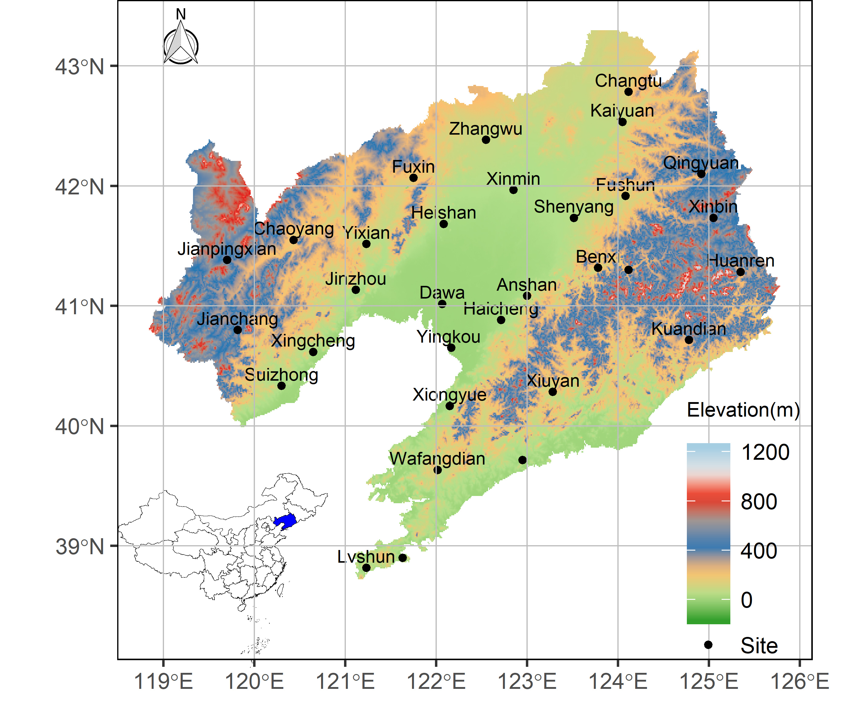
利用R绘制指定区域的DEM图
|||
# 加载运行环境
library(tidyverse)
library(sf)
library(raster)
library(rgdal)
library(glue)
library(data.table)
library(ggsn)
library(cowplot)
## read dem file
myfile <- "00DataSet/dem_250m/dem_250m/w001001.adf"
dem <- new("GDALReadOnlyDataset", myfile) %>% asSGDF_GROD
crs.geo <- CRS("+proj=longlat +ellps=WGS84 +datum=WGS84")
## get the boundary of Three River Plain
sjpy <-
read_sf("00DataSet/Province/CN-sheng-A.shp",
options = "ENCODING=gb2312",
stringsAsFactors = FALSE) %>%
filter(name == "辽宁") %>%
st_transform(crs = crs.geo)
bdf <-sjpy %>% getElement("geometry") %>%
st_transform(crs = crs.geo) %>% as_Spatial()
## mask dem using the boundary
dem.sj <- raster(dem)
dem.sj <- dem.sj %>% crop(bdf) %>%
raster::aggregate(fact = 0.01 / res(dem.sj)) %>% #设置分辨率
mask(bdf) %>% as.data.frame(xy = TRUE)
SitesinRegion <- readRDS("02 DEM/Liaoning/pointsinRegions.rds")
pal8 <- c("#33A02C", "#B2DF8A", "#FDBF6F", "#1F78B4", "#999999", "#E31A1C", "#E6E6E6", "#A6CEE3")
G1 <- ggplot(dem.sj) + geom_raster(aes(x, y, fill = band1), na.rm = TRUE) +
scale_fill_gradientn(colours = pal8, na.value = "transparent")+
geom_point(data = SitesinRegion,aes(x=X,y=Y,size="a"))+
scale_size_manual(
values = c(1),
breaks = c("a"),
labels = c("Site")
) +
geom_text(data = SitesinRegion,
aes(x = X, y = Y, label = EnStationN),
size=2.5,check_overlap =TRUE,nudge_y=0.1) +
north(sjpy,location ="topleft" ,0.1)+
ylim(38.3,43.3)+
coord_sf(crs = crs.geo)+
theme(
plot.background=element_rect(fill = "transparent"),
panel.ontop = TRUE,
panel.background = element_rect(color = NA, fill = NA),
panel.grid=element_line(color = "grey",size = 0.25),
panel.border=element_rect(color = "black",fill = NA ),
legend.key = element_rect(fill=NA,size=0.5,color = NA),
legend.title = element_text(size=8),
legend.position = c(1,0),
legend.justification = c(1,0.08),
legend.spacing.y = unit(-0.2,"cm"),
legend.background = element_rect(fill = "transparent"),
plot.margin = margin(0,0,-0.2,-0.3,"cm")
)+
labs(fill="Elevation(m)",x="",y="",size="")+
guides(size = guide_legend(order=2,title=NULL),
fill=guide_colorbar(order=1,title.vjust=10,barheight =5 ) )
# China mini map ------------------------------------------------------------------------------
China <- read_sf(
"00DataSet/Province/CN-sheng-A.shp",
options = "ENCODING=gb2312",
stringsAsFactors = FALSE
) %>%
st_transform(crs = crs.geo)
G.China <- ggplot(China)+geom_sf(fill="white",color="black",size=0.1)+
geom_sf(data=sjpy,fill="blue",color="black",size=0.1)+
coord_sf(crs = crs.geo)+theme_void()
# insert mini China map into the plot ---------------------------------------------------------
Gs <- cowplot::ggdraw()+
cowplot::draw_grob(ggplotGrob(G.China),x = 0,y = 0,
scale = 0.3,
hjust = 0.24, vjust = 0.3)+
draw_plot(G1)
# draw and preview ----------------------------------------------------------------------------
Taotao::preview.ggplot(Gs,width = 12,height = 10,dpi = 600)
https://m.sciencenet.cn/blog-3427939-1218382.html
下一篇:利用R进行时间序列Mann-Kendall突变检测